Chapter 4. Cohort Analysis
In Chapter 3 we covered time series analysis. With those techniques in hand, we will now turn to a related type of analysis with many business and other applications: cohort analysis.
I remember the first time I encountered a cohort analysis. I was working at my first data analyst job, at a small startup. I was reviewing a purchase analysis I’d worked on with the CEO, and he suggested that I break up the customer base by cohorts to see whether behavior was changing over time. I assumed it was some fancy business school thing and probably useless, but he was the CEO, so of course I humored him. Turns out it wasn’t just a lark. Breaking populations into cohorts and following them over time is a powerful way to analyze your data and avoid various biases. Cohorts can provide clues to how subpopulations differ from each other and how they change over time.
In this chapter, we’ll first take a look at what cohorts are and at the building blocks of certain types of cohort analysis. After an introduction to the legislators data set used for the examples, we’ll learn how to construct a retention analysis and deal with various challenges such as defining the cohort and handling sparse data. Next, we’ll cover survivorship, returnship, and cumulative calculations, all of which are similar to retention analysis in the way the SQL code is structured. Finally, we’ll look at how to combine cohort analysis with cross-sectional analysis to understand the makeup of populations over time.
Cohorts: A Useful Analysis Framework
Before we get into the code, I will define what cohorts are, consider the types of questions we can answer with this type of analysis, and describe the components of any cohort analysis.
A cohort is a group of individuals who share some characteristic of interest, described below, at the time we start observing them. Cohort members are often people but can be any type of entity we want to study: companies, products, or physical world phenomena. Individuals in a cohort may be aware of their membership, just as children in a first-grade class are aware they are part of a peer group of first graders, or participants in a drug trial are aware they are part of a group receiving a treatment. At other times, entities are grouped into cohorts virtually, as when a software company groups all customers acquired in a certain year to study how long they remain customers. It’s always important to consider the ethical implications of cohorting entities without their awareness, if any different treatment is to be applied to them.
Cohort analysis is a useful way to compare groups of entities over time. Many important behaviors take weeks, months, or years to occur or evolve, and cohort analysis is a way to understand these changes. Cohort analysis provides a framework for detecting correlations between cohort characteristics and these long-term trends, which can lead to hypotheses about the causal drivers. For example, customers acquired through a marketing campaign may have different long-term purchase patterns than those who were persuaded by a friend to try a company’s products. Cohort analysis can be used to monitor new cohorts of users or customers and assess how they compare to previous cohorts. Such monitoring can provide an early alert signal that something has gone wrong (or right) for new customers. Cohort analysis is also used to mine historical data. A/B tests, discussed in Chapter 7, are the gold standard for determining causality, but we can’t go back in time and run every test for every question about the past in which we are interested. We should of course be cautious about attaching causal meaning to cohort analysis and instead use cohort analysis as a way to understand customers and generate hypotheses that can be tested rigorously in the future.
Cohort analyses have three components: the cohort grouping, a time series of data over which the cohort is observed, and an aggregate metric that measures an action done by cohort members.
Cohort grouping is often based on a start date: the customer’s first purchase or subscription date, the date a student started school, and so on. However, cohorts can also be formed around other characteristics that are either innate or changing over time. Innate qualities include birth year and country of origin, or the year a company was founded. Characteristics that can change over time include city of residence and marital status. When these are used, we need to be careful to cohort only on the value on the starting date, or else entities can jump between cohort groups.
Cohort or Segment?
These two terms are often used in similar ways, or even interchangeably, but it’s worth drawing a distinction between them for the sake of clarity. A cohort is a group of users (or other entities) who have a common starting date and are followed over time. A segment is a grouping of users who share a common characteristic or set of characteristics at a point in time, regardless of their starting date. Similar to cohorts, segments can be based on innate factors such as age or on behavioral characteristics. A segment of users that signs up in the same month can be put into a cohort and followed over time. Or different groupings of users can be explored with cohort analysis so that you can see which ones have the most valuable characteristics. The analyses we’ll cover in this chapter, such as retention, can help put concrete data behind marketing segments.
The second component of any cohort analysis is the time series. This is a series of purchases, logins, interactions, or other actions that are taken by the customers or entities to be cohorted. It’s important that the time series covers the entire life span of the entities, or there will be survivorship bias in early cohorts. Survivorship bias occurs when only customers who have stayed are in the data set; churned customers are excluded because they are no longer around, so the rest of the customers appear to be of higher quality or fit in comparison to newer cohorts (see “Survivorship Bias”). It’s also important to have a time series that is long enough for the entities to complete the action of interest. For example, if customers tend to purchase once a month, a time series of several months is needed. If, on the other hand, purchases happen only once a year, a time series of several years would be preferable. Inevitably, more recently acquired customers will not have had as long to complete actions as those customers who were acquired further in the past. In order to normalize, cohort analysis usually measures the number of periods that have elapsed from a starting date, rather than calendar months. In this way, cohorts can be compared in period 1, period 2, and so on to see how they evolve over time, regardless of which month the action actually occurred. The intervals may be days, weeks, months, or years.
The aggregate metric should be related to the actions that matter to the health of the organization, such as customers continuing to use or purchase the product. Metric values are aggregated across the cohort, usually with sum, count, or average, though any relevant aggregation works. The result is a time series that can then be used to understand changes in behavior over time.
In this chapter, I’ll cover four types of cohort analysis: retention, survivorship, returnship or repeat purchase behavior, and cumulative behavior.
- Retention
- Retention is concerned with whether the cohort member has a record in the time series on a particular date, expressed as a number of periods from the starting date. This is useful in any kind of organization in which repeated actions are expected, from playing an online game to using a product or renewing a subscription, and it helps to answer questions about how sticky or engaging a product is and how many entities can be expected to appear on future dates.
- Survivorship
- Survivorship is concerned with how many entities remained in the data set for a certain length of time or longer, regardless of the number or frequency of actions up to that time. Survivorship is useful for answering questions about the proportion of the population that can be expected to remain—either in a positive sense by not churning or passing away, or in a negative sense by not graduating or fulfilling some requirement.
- Returnship
- Returnship or repeat purchase behavior is concerned with whether an action has happened more than some minimum threshold of times—often simply more than once—during a fixed window of time. This type of analysis is useful in situations in which the behavior is intermittent and unpredictable, such as in retail, where it characterizes the share of repeat purchasers in each cohort within a fixed time window.
- Cumulative
- Cumulative calculations are concerned with the total number or amounts measured at one or more fixed time windows, regardless of when they happened during that window. Cumulative calculations are often used in calculations of customer lifetime value (LTV or CLTV).
The four types of cohort analysis allow us to compare subgroups and understand how they differ over time in order to make better product, marketing, and financial decisions. The calculations for the different types are similar, so we will set the stage with retention, and then I’ll show how to modify retention code to calculate the other types. Before we dive into constructing our cohort analysis, let’s take a look at the data set we’ll be using for the examples in this chapter.
The Legislators Data Set
The SQL examples in this chapter will use a data set of past and present members of the United States Congress maintained in a GitHub repository. In the US, Congress is responsible for writing laws or legislation, so its members are also known as legislators. Since the data set is a JSON file, I have applied some transformations to produce a more suitable data model for analysis, and I have posted data in a format suitable for following along with the examples in the book’s GitHub legislators folder.
The source repository has an excellent data dictionary, so I won’t repeat all the details here. I will provide a few details, however, that should help those who aren’t familiar with the US government to follow along with the analyses in this chapter.
Congress has two chambers, the Senate (“sen” in the data set) and the House of Representatives (“rep”). Each state has two senators, and they are elected for six-year terms. Representatives are allocated to states based on population; each representative has a district that they alone represent. Representatives are elected for two-year terms. Actual terms in either chamber can be shorter in the event that the legislator dies or is elected or appointed to a higher office. Legislators accumulate power and influence via leadership positions the longer they are in office, and thus standing for re-election is common. Finally, a legislator may belong to a political party, or they may be an “independent.” In the modern era, the vast majority of legislators are Democrats or Republicans, and the rivalry between the two parties is well known. Legislators occasionally change parties while in office.
For the analyses, we’ll make use of two tables: legislators and legislators_terms. The legislators table contains a list of all the people included in the data set, with birthday, gender, and a set of ID fields that can be used to look up the person in other data sets. The legislators_terms table contains a record for each term in office for each legislator, with start and end date, and other attributes such as chamber and party. The id_bioguide field is used as the unique identifier of a legislator and appears in each table. Figure 4-1 shows a sample of the legislators data. Figure 4-2 shows a sample of the legislators_terms data.
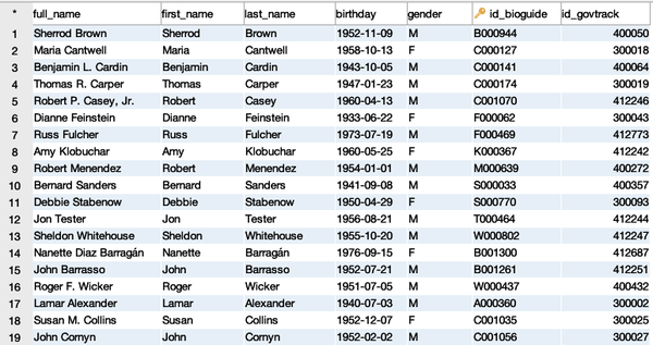
Figure 4-1. Sample of the legislators table
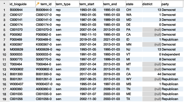
Figure 4-2. Sample of the legislators_terms table
Now that we have an understanding of what cohort analysis is and of the data set we’ll be using for examples, let’s get into how to write SQL for retention analysis. The key question SQL will help us answer is: once representatives take office, how long do they keep their jobs?
Retention
One of the most common types of cohort analysis is retention analysis. To retain is to keep or continue something. Many skills need to be practiced to be retained. Businesses usually want their customers to keep purchasing their products or using their services, since retaining customers is more profitable than acquiring new ones. Employers want to retain their employees, because recruiting replacements is expensive and time consuming. Elected officials seek reelection in order to continue working on the priorities of their constituents.
The main question in retention analysis is whether the starting size of the cohort—number of subscribers or employees, amount spent, or another key metric—will remain constant, decay, or increase over time. When there is an increase or a decrease, the amount and speed of change are also interesting questions. In most retention analyses, the starting size will tend to decay over time, since a cohort can lose but cannot gain new members once it is formed. Revenue is an interesting exception, since a cohort of customers can spend more in subsequent months than they did in the first month collectively, even if some of them churn.
Retention analysis uses the count of entities or sum of money or actions present in the data set for each period from the starting date, and it normalizes by dividing this number by the count or sum of entities, money, or actions in the first time period. The result is expressed as a percentage, and retention in the starting period is always 100%. Over time, retention based on counts generally declines and can never exceed 100%, whereas money- or action-based retention, while often declining, can increase and be greater than 100% in a time period. Retention analysis output is typically displayed in either table or graph form, which is referred to as a retention curve. We’ll see a number of examples of retention curves later in this chapter.
Graphs of retention curves can be used to compare cohorts. The first characteristic to pay attention to is the shape of the curve in the initial few periods, where there is often an initial steep drop. For many consumer apps, losing half a cohort in the first few months is common. A cohort with a curve that is either more or less steep than others can indicate changes in the product or customer acquisition source that merit further investigation. A second characteristic to look for is whether the curve flattens after some number of periods or continues declining rapidly to zero. A flattening curve indicates that there is a point in time from which most of the cohort that remains stays indefinitely. A retention curve that inflects upward, sometimes called a smile curve, can occur if cohort members return or reactivate after falling out of the data set for some period. Finally, retention curves that measure subscription revenue are monitored for signs of increasing revenue per customer over time, a sign of a healthy SaaS software business.
This section will show how to create a retention analysis, add cohort groupings from the time series itself and other tables, and handle missing and sparse data that can occur in time series data. With this framework in hand, you’ll learn in the subsequent section how to make modifications to create the other related types of cohort analysis. As a result, this section on retention will be the longest one in the chapter, as you build up code and develop your intuition about the calculations.
SQL for a Basic Retention Curve
For retention analysis, as with other cohort analyses, we need three components: the cohort definition, a time series of actions, and an aggregate metric that measures something relevant to the organization or process. In our case, the cohort members will be the legislators, the time series will be the terms in office for each legislator, and the metric of interest will be the count of those who are still in office each period from the starting date.
We’ll start by calculating basic retention, before moving on to examples that include various cohort groupings. The first step is to find the first date each legislator took office (first_term). We will use this date to calculate the number of periods for each subsequent date in the time series. To do this, take the min of the term_start and GROUP BY each id_bioguide, the unique identifier for a legislator:
SELECT id_bioguide
,min(term_start) as first_term
FROM legislators_terms
GROUP BY 1
;

id_bioguide  first_term
-----------  ----------
A000118      1975-01-14
P000281      1933-03-09
K000039      1933-03-09
...          ...
The next step is to put this code into a subquery and JOIN it to the time series. The age function is applied to calculate the intervals between each term_start and the first_term for each legislator. Applying the date_part functions to the result, with year, transforms this into the number of yearly periods. Since elections happen every two or six years, we’ll use years as the time interval to calculate the periods. We could use a shorter interval, but in this data set there is little fluctuation daily or weekly. The count of legislators with records for that period is the number retained:
SELECT date_part('year',age(b.term_start,a.first_term)) as period
,count(distinct a.id_bioguide) as cohort_retained
FROM
(
    SELECT id_bioguide, min(term_start) as first_term
    FROM legislators_terms
    GROUP BY 1
) a
JOIN legislators_terms b on a.id_bioguide = b.id_bioguide
GROUP BY 1
;

period  cohort_retained
------  ---------------
0.0     12518
1.0     3600
2.0     3619
...     ...
Tip
In databases that support the datediff function, the date_part and age construction can be replaced by this simpler function:
datediff('year',first_term,term_start)
Some databases, such as Oracle, place the date_part last:
datediff(first_term,term_start,'year'
Now that we have the periods and the number of legislators retained in each, the final step is to calculate the total cohort_size and populate it in each row so that the cohort_retained can be divided by it. The first_value window function returns the first record in the PARTITION BY clause, according to the ordering set in the ORDER BY, a convenient way to get the cohort size in each row. In this case, the cohort_size comes from the first record in the entire data set, so the PARTITION BY is omitted:
first_value(cohort_retained) over (order by period) as cohort_size
To find the percent retained, divide the cohort_retained value by this same calculation:
SELECT period
,first_value(cohort_retained) over (order by period) as cohort_size
,cohort_retained
,cohort_retained /
 first_value(cohort_retained) over (order by period) as pct_retained
FROM
(
    SELECT date_part('year',age(b.term_start,a.first_term)) as period
    ,count(distinct a.id_bioguide) as cohort_retained
    FROM
    (
        SELECT id_bioguide, min(term_start) as first_term
        FROM legislators_terms
        GROUP BY 1
    ) a
    JOIN legislators_terms b on a.id_bioguide = b.id_bioguide
    GROUP BY 1
) aa
;

period  cohort_size  cohort_retained  pct_retained
------  -----------  ---------------  ------------
0.0     12518        12518            1.0000
1.0     12518        3600             0.2876
2.0     12518        3619             0.2891
...     ...          ...              ...
We now have a retention calculation, and we can see that there is a big drop-off between the 100% of legislators retained in period 0, or on their start date, and the share with another term record that starts a year later. Graphing the results, as in Figure 4-3, demonstrates how the curve flattens and eventually goes to zero, as even the longest-serving legislators eventually retire or die.
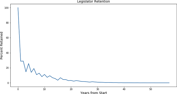
Figure 4-3. Retention from start of first term for US legislators
We can take the cohort retention result and reshape the data to show it in table format. Pivot and flatten the results using an aggregate function with a CASE statement; max is used in this example, but other aggregations such as min or avg would return the same result. Retention is calculated for years 0 through 4, but additional years can be added by following the same pattern:
SELECT cohort_size
,max(case when period = 0 then pct_retained end) as yr0
,max(case when period = 1 then pct_retained end) as yr1
,max(case when period = 2 then pct_retained end) as yr2
,max(case when period = 3 then pct_retained end) as yr3
,max(case when period = 4 then pct_retained end) as yr4
FROM
(
    SELECT period
    ,first_value(cohort_retained) over (order by period)
     as cohort_size
    ,cohort_retained
     / first_value(cohort_retained) over (order by period)
     as pct_retained
    FROM
    (
        SELECT
        date_part('year',age(b.term_start,a.first_term)) as period
        ,count(*) as cohort_retained
        FROM
        (
            SELECT id_bioguide, min(term_start) as first_term
            FROM legislators_terms
            GROUP BY 1
        ) a
        JOIN legislators_terms b on a.id_bioguide = b.id_bioguide
        GROUP BY 1
    ) aa
) aaa
GROUP BY 1
;

cohort_size  yr0     yr1     yr2     yr3     yr4
-----------  ------  ------  ------  ------  ------
12518        1.0000  0.2876  0.2891  0.1463  0.2564
Retention appears to be quite low, and from the graph we can see that it is jagged in the first few years. One reason for this is that a representative’s term lasts two years, and senators’ terms last six years, but the data set only contains records for the start of new terms; thus we are missing data for years in which a legislator was still in office but did not start a new term. Measuring retention each year is misleading in this case. One option is to measure retention only on a two- or six-year cycle, but there is also another strategy we can employ to fill in the “missing” data. I will cover this next before returning to the topic of forming cohort groups.
Adjusting Time Series to Increase Retention Accuracy
We discussed techniques for cleaning “missing” data in Chapter 2, and we will turn to those techniques in this section in order to arrive at a smoother and more truthful retention curve for the legislators. When working with time series data, such as in cohort analysis, it’s important to consider not only the data that is present but also whether that data accurately reflects the presence or absence of entities at each time period. This is particularly a problem in contexts in which an event captured in the data leads to the entity persisting for some period of time that is not captured in the data. For example, a customer buying a software subscription is represented in the data at the time of the transaction, but that customer is entitled to use the software for months or years and is not necessarily represented in the data over that span. To correct for this, we need a way to derive the span of time in which the entity is still present, either with an explicit end date or with knowledge of the length of the subscription or term. Then we can say that the entity was present at any date in between those start and end dates.
In the legislators data set, we have a record for a term’s start date, but we are missing the notion that this “entitles” a legislator to serve for two or six years, depending on the chamber. To correct for this and smooth out the curve, we need to fill in the “missing” values for the years that legislators are still in office between new terms. Since this data set includes a term_end value for each term, I’ll show how to create a more accurate cohort retention analysis by filling in dates between the start and end values. Then I’ll show how you can impute end dates when the data set does not include an end date.
Calculating retention using a start and end date defined in the data is the most accurate approach. For the following examples, we will consider legislators retained in a particular year if they were still in office as of the last day of the year, December 31. Prior to the Twentieth Amendment to the US Constitution, terms began on March 4, but afterward the start date moved to January 3, or to a subsequent weekday if the third falls on a weekend. Legislators can be sworn in on other days of the year due to special off-cycle elections or appointments to fill vacant seats. As a result, term_start dates cluster in January but are spread across the year. While we could pick another day, December 31 is a strategy for normalizing around these varying start dates.
The first step is to create a data set that contains a record for each December 31 that each legislator was in office. This can be accomplished by JOINing the subquery that found the first_term to the legislators_terms table to find the term_start and term_end for each term. A second JOIN to the date_dim retrieves the dates that fall between the start and end dates, restricting the returned values to c.month_name = 'December' and c.day_of_month = 31. The period is calculated as the years between the date from the date_dim and the first_term. Note that even though more than 11 months may have elapsed between being sworn in in January and December 31, the first year still appears as 0:
SELECT a.id_bioguide, a.first_term
,b.term_start, b.term_end
,c.date
,date_part('year',age(c.date,a.first_term)) as period
FROM
(
    SELECT id_bioguide, min(term_start) as first_term
    FROM legislators_terms
    GROUP BY 1
) a
JOIN legislators_terms b on a.id_bioguide = b.id_bioguide
LEFT JOIN date_dim c on c.date between b.term_start and b.term_end
and c.month_name = 'December' and c.day_of_month = 31
;

id_bioguide  first_term  term_start  term_end    date        period
-----------  ----------  ----------  ----------  ----------  ------
B000944      1993-01-05  1993-01-05  1995-01-03  1993-12-31  0.0
B000944      1993-01-05  1993-01-05  1995-01-03  1994-12-31  1.0
C000127      1993-01-05  1993-01-05  1995-01-03  1993-12-31  0.0
...          ...         ...         ...         ...         ...
Tip
If a date dimension is not available, you can create a subquery with the necessary dates in a couple of ways. If your database supports the generate_series, you can create a subquery that returns the desired dates:
SELECT generate_series::date as date
FROM generate_series('1770-12-31','2020-12-
31',interval '1 year')
You may want to save this as a table or view for later use. Alternatively, you can query the data set or any other table in the database that has a full set of dates. In this case, the table has all of the necessary years, but we will make a December 31 date for each year using the make_date function:
SELECT distinct
make_date(date_part('year',term_start)::int,12,31)
FROM legislators_terms
There are a number of creative ways to get the series of dates needed. Use whichever method is available and simplest within your queries.
We now have a row for each date (year end) for which we would like to calculate retention. The next step is to calculate the cohort_retained for each period, which is done with a count of id_bioguide. A coalesce function is used on period to set a default value of 0 when null. This handles the cases in which a legislator’s term starts and ends in the same year, giving credit for serving in that year:
SELECT
coalesce(date_part('year',age(c.date,a.first_term)),0) as period
,count(distinct a.id_bioguide) as cohort_retained
FROM
(
    SELECT id_bioguide, min(term_start) as first_term
    FROM legislators_terms
    GROUP BY 1
) a
JOIN legislators_terms b on a.id_bioguide = b.id_bioguide
LEFT JOIN date_dim c on c.date between b.term_start and b.term_end
and c.month_name = 'December' and c.day_of_month = 31
GROUP BY 1
;

period  cohort_retained
------  ---------------
0.0     12518
1.0     12328
2.0     8166
...     ...
The final step is to calculate the cohort_size and pct_retained as we did previously using first_value window functions:
SELECT period
,first_value(cohort_retained) over (order by period) as cohort_size
,cohort_retained
,cohort_retained * 1.0 /
 first_value(cohort_retained) over (order by period) as pct_retained
FROM
(
    SELECT coalesce(date_part('year',age(c.date,a.first_term)),0) as period
    ,count(distinct a.id_bioguide) as cohort_retained
    FROM
    (
        SELECT id_bioguide, min(term_start) as first_term
        FROM legislators_terms
        GROUP BY 1
    ) a
    JOIN legislators_terms b on a.id_bioguide = b.id_bioguide
    LEFT JOIN date_dim c on c.date between b.term_start and b.term_end
    and c.month_name = 'December' and c.day_of_month = 31
    GROUP BY 1
) aa
;

period  cohort_size  cohort_retained  pct_retained
------  -----------  ---------------  ------------
0.0     12518        12518            1.0000
1.0     12518        12328            0.9848
2.0     12518        8166             0.6523
...     ...          ...              ...
The results, graphed in Figure 4-4, are now much more accurate. Almost all legislators are still in office in year 1, and the first big drop-off occurs in year 2, when some representatives will fail to be reelected.
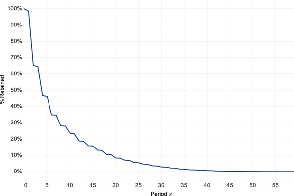
Figure 4-4. Legislator retention after adjusting for actual years in office
If the data set does not contain an end date, there are a couple of options for imputing one. One option is to add a fixed interval to the start date, when the length of a subscription or term is known. This can be done with date math by adding a constant interval to the term_start. Here, a CASE statement handles the addition for the two term_types:
SELECT a.id_bioguide, a.first_term
,b.term_start
,case when b.term_type = 'rep' then b.term_start + interval '2 years'
      when b.term_type = 'sen' then b.term_start + interval '6 years'
      end as term_end
FROM
(
    SELECT id_bioguide, min(term_start) as first_term
    FROM legislators_terms
    GROUP BY 1
) a
JOIN legislators_terms b on a.id_bioguide = b.id_bioguide
;

id_bioguide  first_term  term_start  term_end
-----------  ----------  ----------  ----------
B000944      1993-01-05  1993-01-05  1995-01-05
C000127      1993-01-05  1993-01-05  1995-01-05
C000141      1987-01-06  1987-01-06  1989-01-06
...          ...         ...         ...
This block of code can then be plugged into the retention code to derive the period and pct_retained. The drawback to this method is that it fails to capture instances in which a legislator did not complete a full term, which can happen in the event of death or appointment to a higher office.
A second option is to use the subsequent starting date, minus one day, as the term_end date. This can be calculated with the lead window function. This function is similar to the lag function we’ve used previously, but rather than returning a value from a row earlier in the partition, it returns a value from a row later in the partition, as determined in the ORDER BY clause. The default is one row, which we will use here, but the function has an optional argument indicating a different number of rows. Here we find the term_start date of the subsequent term using lead and then subtract the interval '1 day' to derive the term_end:
SELECT a.id_bioguide, a.first_term
,b.term_start
,lead(b.term_start) over (partition by a.id_bioguide
                          order by b.term_start)
 - interval '1 day' as term_end
FROM
(
    SELECT id_bioguide, min(term_start) as first_term
    FROM legislators_terms
    GROUP BY 1
) a
JOIN legislators_terms b on a.id_bioguide = b.id_bioguide
;

id_bioguide  first_term  term_start  term_end
-----------  ----------  ----------  ----------
A000001      1951-01-03  1951-01-03  (null)
A000002      1947-01-03  1947-01-03  1949-01-02
A000002      1947-01-03  1949-01-03  1951-01-02
...          ...         ...         ...
This code block can then be plugged into the retention code. This method has a couple of drawbacks. First, when there is no subsequent term, the lead function returns null, leaving that term without a term_end. A default value, such as a default interval shown in the last example, could be used in such cases. The second drawback is that this method assumes that terms are always consecutive, with no time spent out of office. Although most legislators tend to serve continuously until their congressional careers end, there are certainly examples of gaps between terms spanning several years.
Any time we make adjustments to fill in missing data, we need to be careful about the assumptions we make. In subscription- or term-based contexts, explicit start and end dates tend to be most accurate. Either of the two other methods shown—adding a fixed interval or setting the end date relative to the next start date—can be used when no end date is present and we have a reasonable expectation that most customers or users will stay for the duration assumed.
Now that we’ve seen how to calculate a basic retention curve and correct for missing dates, we can start adding in cohort groups. Comparing retention between different groups is one of the main reasons to do cohort analysis. Next, I’ll discuss forming groups from the time series itself, and after that, I’ll discuss forming cohort groups from data in other tables.
Cohorts Derived from the Time Series Itself
Now that we have SQL code to calculate retention, we can start to split the entities into cohorts. In this section, I will show how to derive cohort groupings from the time series itself. First I’ll discuss time-based cohorts based on the first date, and I’ll explain how to make cohorts based on other attributes from the time series.
The most common way to create the cohorts is based on the first or minimum date or time that the entity appears in the time series. This means that only one table is necessary for the cohort retention analysis: the time series itself. Cohorting by the first appearance or action is interesting because often groups that start at different times behave differently. For consumer services, early adopters are often more enthusiastic and retain differently than later adopters, whereas in SaaS software, later adopters may retain better because the product is more mature. Time-based cohorts can be grouped by any time granularity that is meaningful to the organization, though weekly, monthly, or yearly cohorts are common. If you’re not sure what grouping to use, try running the cohort analysis with different groupings, without making the cohort sizes too small, to see where meaningful patterns emerge. Fortunately, once you know how to construct the cohorts and retention analysis, substituting different time granularities is straightforward.
The first example will use yearly cohorts, and then I will demonstrate swapping in centuries. The key question we will consider is whether the era in which a legislator first took office has any correlation with their retention. Political trends and the public mood do change over time, but by how much?
To calculate yearly cohorts, we first add the year of the first_term calculated previously to the query that finds the period and cohort_retained:
SELECT date_part('year',a.first_term) as first_year
,coalesce(date_part('year',age(c.date,a.first_term)),0) as period
,count(distinct a.id_bioguide) as cohort_retained
FROM
(
    SELECT id_bioguide, min(term_start) as first_term
    FROM legislators_terms
    GROUP BY 1
) a
JOIN legislators_terms b on a.id_bioguide = b.id_bioguide
LEFT JOIN date_dim c on c.date between b.term_start and b.term_end
and c.month_name = 'December' and c.day_of_month = 31
GROUP BY 1,2
;

first_year  period  cohort_retained
----------  ------  ---------------
1789.0      0.0     89
1789.0      2.0     89
1789.0      3.0     57
...         ...     ...
This query is then used as the subquery, and the cohort_size and pct_retained are calculated in the outer query as previously. In this case, however, we need a PARTITION BY clause that includes first_year so that the first_value is calculated only within the set of rows for that first_year, rather than across the whole result set from the subquery:
SELECT first_year, period
,first_value(cohort_retained) over (partition by first_year
                                    order by period) as cohort_size
,cohort_retained
,cohort_retained /
 first_value(cohort_retained) over (partition by first_year
                                    order by period) as pct_retained
FROM
(
    SELECT date_part('year',a.first_term) as first_year
    ,coalesce(date_part('year',age(c.date,a.first_term)),0) as period
    ,count(distinct a.id_bioguide) as cohort_retained
    FROM
    (
        SELECT id_bioguide, min(term_start) as first_term
        FROM legislators_terms
        GROUP BY 1
    ) a
    JOIN legislators_terms b on a.id_bioguide = b.id_bioguide
    LEFT JOIN date_dim c on c.date between b.term_start and b.term_end
    and c.month_name = 'December' and c.day_of_month = 31
    GROUP BY 1,2
) aa
;

first_year  period  cohort_size  cohort_retained  pct_retained
----------  ------  -----------  ---------------  ------------
1789.0      0.0     89           89               1.0000
1789.0      2.0     89           89               1.0000
1789.0      3.0     89           57               0.6404
...         ...     ...          ...              ...
This data set includes over two hundred starting years, too many to easily graph or examine in a table. Next we’ll look at a less granular interval and cohort the legislators by the century of the first_term. This change is easily made by substituting century for year in the date_part function in subquery aa. Recall that century names are offset from the years they represent, so that the 18th century lasted from 1700 to 1799, the 19th century lasted from 1800 to 1899, and so on. The partitioning in the first_value function changes to the first_century field:
SELECT first_century, period
,first_value(cohort_retained) over (partition by first_century
                                    order by period) as cohort_size
,cohort_retained
,cohort_retained /
 first_value(cohort_retained) over (partition by first_century
                                    order by period) as pct_retained
FROM
(
    SELECT date_part('century',a.first_term) as first_century
    ,coalesce(date_part('year',age(c.date,a.first_term)),0) as period
    ,count(distinct a.id_bioguide) as cohort_retained
    FROM
    (
        SELECT id_bioguide, min(term_start) as first_term
        FROM legislators_terms
        GROUP BY 1
    ) a
    JOIN legislators_terms b on a.id_bioguide = b.id_bioguide
    LEFT JOIN date_dim c on c.date between b.term_start and b.term_end
    and c.month_name = 'December' and c.day_of_month = 31
    GROUP BY 1,2
) aa
ORDER BY 1,2
;

first_century  period  cohort_size  cohort_retained  pct_retained
-------------  ------  -----------  ---------------  ------------
18.0           0.0     368          368              1.0000
18.0           1.0     368          360              0.9783
18.0           2.0     368          242              0.6576
...            ...     ...          ...              ...
The results are graphed in Figure 4-5. Retention in the early years has been higher for those first elected in the 20th or 21st century. The 21st century is still underway, and thus many of those legislators have not had the opportunity to stay in office for five or more years, though they are still included in the denominator. We might want to consider removing the 21st century from the analysis, but I’ve left it here to demonstrate how the retention curve drops artificially due to this circumstance.
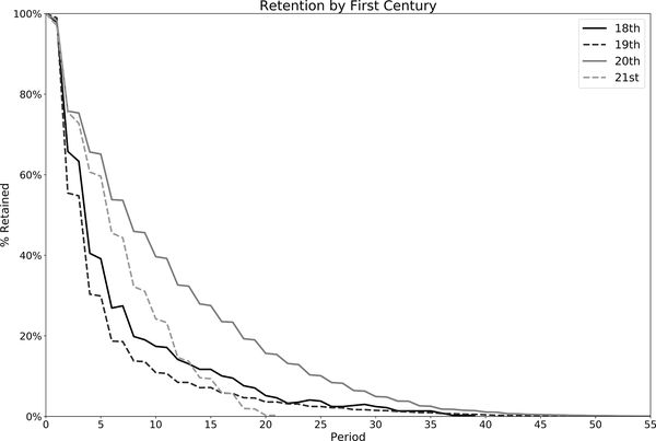
Figure 4-5. Legislator retention by century in which first term began
Cohorts can be defined from other attributes in a time series besides the first date, with options depending on the values in the table. The legislators_terms table has a state field, indicating which state the person is representing for that term. We can use this to create cohorts, and we will base them on the first state in order to ensure that anyone who has represented multiple states appears in the data only once.
Warning
When cohorting on an attribute that can change over time, it’s important to ensure that each entity is assigned only one value. Otherwise the entity may be represented in multiple cohorts, introducing bias into the analysis. Usually the value from the earliest record in the data set is used.
To find the first state for each legislator, we can use the first_value window function. In this example, we’ll also turn the min function into a window function to avoid a lengthy GROUP BY clause:
SELECT distinct id_bioguide
,min(term_start) over (partition by id_bioguide) as first_term
,first_value(state) over (partition by id_bioguide
                          order by term_start) as first_state
FROM legislators_terms
;

id_bioguide  first_term  first_state
-----------  ----------  -----------
C000001      1893-08-07  GA
R000584      2009-01-06  ID
W000215      1975-01-14  CA
...          ...         ...
We can then plug this code into our retention code to find the retention by first_state:
SELECT first_state, period
,first_value(cohort_retained) over (partition by first_state
                                    order by period) as cohort_size
,cohort_retained
,cohort_retained /
 first_value(cohort_retained) over (partition by first_state
                                    order by period) as pct_retained
FROM
(
    SELECT a.first_state
    ,coalesce(date_part('year',age(c.date,a.first_term)),0) as period
    ,count(distinct a.id_bioguide) as cohort_retained
    FROM
    (
        SELECT distinct id_bioguide
        ,min(term_start) over (partition by id_bioguide) as first_term
        ,first_value(state) over (partition by id_bioguide order by term_start)
         as first_state
        FROM legislators_terms
    ) a
    JOIN legislators_terms b on a.id_bioguide = b.id_bioguide
    LEFT JOIN date_dim c on c.date between b.term_start and b.term_end
    and c.month_name = 'December' and c.day_of_month = 31
    GROUP BY 1,2
) aa
;

first_state  period  cohort_size  cohort_retained  pct_retained
-----------  ------  -----------  ---------------  ------------
AK           0.0     19           19               1.0000
AK           1.0     19           19               1.0000
AK           2.0     19           15               0.7895
...          ...     ...          ...              ...
The retention curves for the five states with the highest total number of legislators are graphed in Figure 4-6. Those elected in Illinois and Massachusetts have the highest retention, while New Yorkers have the lowest retention. Determining the reasons why would be an interesting offshoot of this analysis.
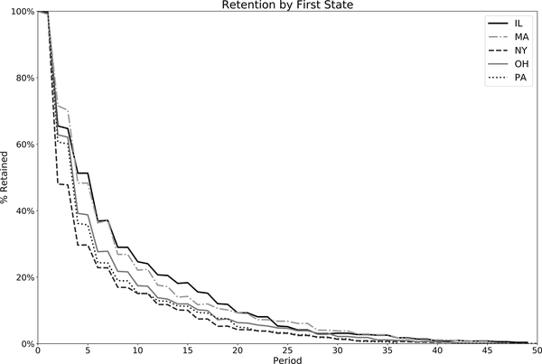
Figure 4-6. Legislator retention by first state: top five states by total legislators
Defining cohorts from the time series is relatively straightforward using a min date for each entity and then converting that date into a month, year, or century as appropriate for the analysis. Switching between month and year or other levels of granularity also is straightforward, allowing for multiple options to be tested in order to find a grouping that is meaningful for the organization. Other attributes can be used for cohorting with the first_value window function. Next, we’ll turn to cases in which the cohorting attribute comes from a table other than that of the time series.
Defining the Cohort from a Separate Table
Often the characteristics that define a cohort exist in a table separate from the one that contains the time series. For example, a database might have a customer table with information such as acquisition source or registration date by which customers can be cohorted. Adding in attributes from other tables, or even subqueries, is relatively straightforward and can be done in retention analysis and related analyses discussed later in the chapter.
For this example, we’ll consider whether the gender of the legislator has any impact on their retention. The legislators table has a gender field, where F means female and M means male, that we can use to cohort the legislators. To do this, we’ll JOIN the legislators table in as alias d to add gender to the calculation of cohort_retained, in place of year or century:
SELECT d.gender
,coalesce(date_part('year',age(c.date,a.first_term)),0) as period
,count(distinct a.id_bioguide) as cohort_retained
FROM
(
    SELECT id_bioguide, min(term_start) as first_term
    FROM legislators_terms
    GROUP BY 1
) a
JOIN legislators_terms b on a.id_bioguide = b.id_bioguide
LEFT JOIN date_dim c on c.date between b.term_start and b.term_end
and c.month_name = 'December' and c.day_of_month = 31
JOIN legislators d on a.id_bioguide = d.id_bioguide
GROUP BY 1,2
;

gender  period  cohort_retained
------  ------  ---------------
F       0.0     366
M       0.0     12152
F       1.0     349
M       1.0     11979
...     ...     ...
It’s immediately clear that many more males than females have served legislative terms. We can now calculate the percent_retained so we can compare the retention for these groups:
SELECT gender, period
,first_value(cohort_retained) over (partition by gender
                                    order by period) as cohort_size
,cohort_retained
,cohort_retained/
 first_value(cohort_retained) over (partition by gender
                                    order by period) as pct_retained
FROM
(
    SELECT d.gender
    ,coalesce(date_part('year',age(c.date,a.first_term)),0) as period
    ,count(distinct a.id_bioguide) as cohort_retained
    FROM
    (
        SELECT id_bioguide, min(term_start) as first_term
        FROM legislators_terms
        GROUP BY 1
    ) a
    JOIN legislators_terms b on a.id_bioguide = b.id_bioguide
    LEFT JOIN date_dim c on c.date between b.term_start and b.term_end
    and c.month_name = 'December' and c.day_of_month = 31
    JOIN legislators d on a.id_bioguide = d.id_bioguide
    GROUP BY 1,2
) aa
;

gender  period  cohort_size  cohort_retained  pct_retained
------  ------  -----------  ---------------  ------------
F       0.0     366          366              1.0000
M       0.0     12152        12152            1.0000
F       1.0     366          349              0.9536
M       1.0     12152        11979            0.9858
...     ...     ...          ...              ...
We can see from the results graphed in Figure 4-7 that retention is higher for female legislators than for their male counterparts for periods 2 through 29. The first female legislator did not take office until 1917, when Jeannette Rankin joined the House as a Republican representative from Montana. As we saw earlier, retention has increased in more recent centuries.
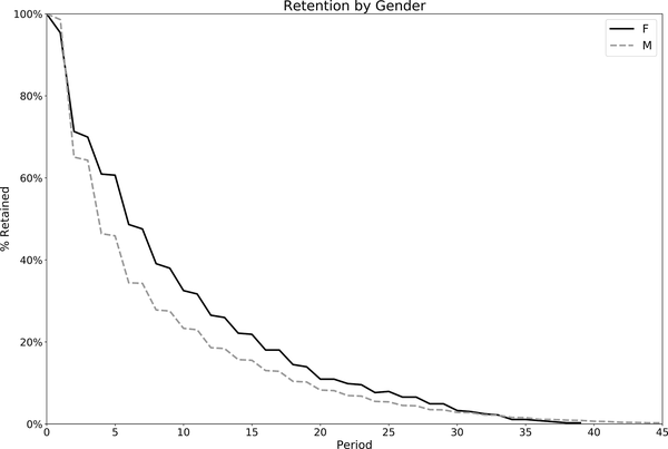
Figure 4-7. Legislator retention by gender
To make a more fair comparison, we might restrict the legislators included in the analysis to only those whose first_term started since there have been women in Congress. We can do this by adding a WHERE filter to subquery aa. Here the results are also restricted to those who started before 2000, to ensure the cohorts have had at least 20 possible years to stay in office:
SELECT gender, period
,first_value(cohort_retained) over (partition by gender
                                    order by period) as cohort_size
,cohort_retained
,cohort_retained /
 first_value(cohort_retained) over (partition by gender
                                    order by period) as pct_retained
FROM
(
    SELECT d.gender
    ,coalesce(date_part('year',age(c.date,a.first_term)),0) as period
    ,count(distinct a.id_bioguide) as cohort_retained
    FROM
    (
        SELECT id_bioguide, min(term_start) as first_term
        FROM legislators_terms
        GROUP BY 1
    ) a
    JOIN legislators_terms b on a.id_bioguide = b.id_bioguide
    LEFT JOIN date_dim c on c.date between b.term_start and b.term_end
    and c.month_name = 'December' and c.day_of_month = 31
    JOIN legislators d on a.id_bioguide = d.id_bioguide
    WHERE a.first_term between '1917-01-01' and '1999-12-31'
    GROUP BY 1,2
) aa
;

gender  period  cohort_size  cohort_retained  pct_retained
------  ------  -----------  ---------------  ------------
F       0.0     200          200              1.0000
M       0.0     3833         3833             1.0000
F       1.0     200          187              0.9350
M       1.0     3833         3769             0.9833
...     ...     ...          ...              ...
Male legislators still outnumber female legislators, but by a smaller margin. The retention for the cohorts is graphed in Figure 4-8. With the revised cohorts, male legislators have higher retention through year 7, but starting in year 12, female legislators have higher retention. The difference between the two gender-based cohort analyses underscores the importance of setting up appropriate cohorts and ensuring that they have comparable amounts of time to be present or complete other actions of interest. To further improve this analysis, we could cohort by both starting year or decade and gender, in order to control for additional changes in retention through the 20th century and into the 21st century.
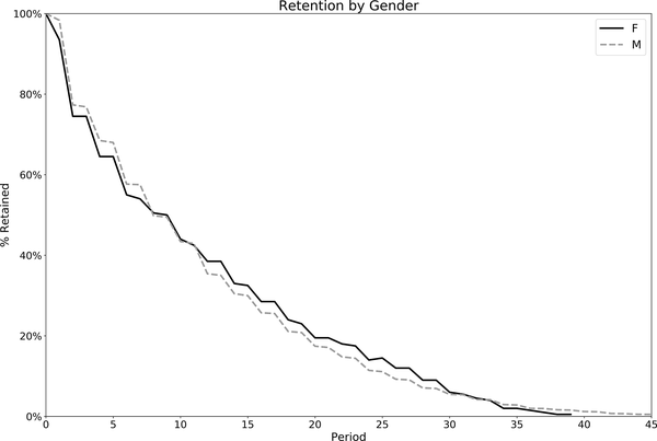
Figure 4-8. Legislator retention by gender: cohorts from 1917 to 1999
Cohorts can be defined in multiple ways, from the time series and from other tables. With the framework we’ve developed, subqueries, views, or other derived tables can be swapped in, opening up a whole range of calculations to be the basis of a cohort. Multiple criteria, such as starting year and gender, can be used. One caution when dividing populations into cohorts based on multiple criteria is that this can lead to sparse cohorts, where some of the defined groups are too small and are not represented in the data set for all time periods. The next section will discuss methods for overcoming this challenge.
Dealing with Sparse Cohorts
In the ideal data set, every cohort has some action or record in the time series for every period of interest. We’ve already seen how “missing” dates can occur due to subscriptions or terms lasting over multiple periods, and we looked at how to correct for them using a date dimension to infer intermediate dates. Another issue can arise when, due to grouping criteria, the cohort becomes too small and as a result is represented only sporadically in the data. A cohort may disappear from the result set, when we would prefer it to appear with a zero retention value. This problem is called sparse cohorts, and it can be worked around with the careful use of LEFT JOINs.
To demonstrate this, let’s attempt to cohort female legislators by the first state they represented to see if there are any differences in retention. We’ve already seen that there have been relatively few female legislators. Cohorting them further by state is highly likely to create some sparse cohorts in which there are very few members. Before making code adjustments, let’s add first_state (calculated in the section on deriving cohorts from the time series) into our previous gender example and look at the results:
SELECT first_state, gender, period
,first_value(cohort_retained) over (partition by first_state, gender
                                    order by period) as cohort_size
,cohort_retained
,cohort_retained /
 first_value(cohort_retained) over (partition by first_state, gender
                                    order by period) as pct_retained
FROM
(
    SELECT a.first_state, d.gender
    ,coalesce(date_part('year',age(c.date,a.first_term)),0) as period
    ,count(distinct a.id_bioguide) as cohort_retained
    FROM
    (
        SELECT distinct id_bioguide
        ,min(term_start) over (partition by id_bioguide) as first_term
        ,first_value(state) over (partition by id_bioguide
                                  order by term_start) as first_state
        FROM legislators_terms
    ) a
    JOIN legislators_terms b on a.id_bioguide = b.id_bioguide
    LEFT JOIN date_dim c on c.date between b.term_start and b.term_end
    and c.month_name = 'December' and c.day_of_month = 31
    JOIN legislators d on a.id_bioguide = d.id_bioguide
    WHERE a.first_term between '1917-01-01' and '1999-12-31'
    GROUP BY 1,2,3
) aa
;


first_state  gender  period  cohort_size  cohort_retained pct_retained
-----------  ------  ------  -----------  --------------- ------------
AZ           F       0.0     2            2               1.0000
AZ           M       0.0     26           26              1.0000
AZ           F       1.0     2            2               1.0000
...          ...     ...     ...          ...             ...
Graphing the results for the first 20 periods, as in Figure 4-9, reveals the sparse cohorts. Alaska did not have any female legislators, while Arizona’s female retention curve disappears after year 3. Only California, a large state with many legislators, has complete retention curves for both genders. This pattern repeats for other small and large states.
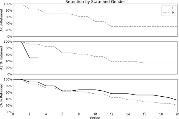
Figure 4-9. Legislator retention by gender and first state
Now let’s look at how to ensure a record for every period so that the query returns zero values for retention instead of nulls. The first step is to query for all combinations of periods and cohort attributes, in this case first_state and gender, with the starting cohort_size for each combination. This can be done by JOINing subquery aa, which calculates the cohort, with a generate_series subquery that returns all integers from 0 to 20, with the criteria on 1 = 1. This is a handy way to force a Cartesian JOIN when the two subqueries don’t have any fields in common:
SELECT aa.gender, aa.first_state, cc.period, aa.cohort_size
FROM
(
    SELECT b.gender, a.first_state
    ,count(distinct a.id_bioguide) as cohort_size
    FROM
    (
        SELECT distinct id_bioguide
        ,min(term_start) over (partition by id_bioguide) as first_term
        ,first_value(state) over (partition by id_bioguide
                                  order by term_start) as first_state
        FROM legislators_terms
    ) a
    JOIN legislators b on a.id_bioguide = b.id_bioguide
    WHERE a.first_term between '1917-01-01' and '1999-12-31'
    GROUP BY 1,2
) aa
JOIN
(
    SELECT generate_series as period
    FROM generate_series(0,20,1)
) cc on 1 = 1
;

gender  state  period  cohort
------  -----  ------  ------
F       AL     0       3
F       AL     1       3
F       AL     2       3
...    ...     ...     ...
The next step is to JOIN this back to the actual periods in office, with a LEFT JOIN to ensure all the time periods remain in the final result:
SELECT aaa.gender, aaa.first_state, aaa.period, aaa.cohort_size
,coalesce(ddd.cohort_retained,0) as cohort_retained
,coalesce(ddd.cohort_retained,0) / aaa.cohort_size as pct_retained
FROM
(
    SELECT aa.gender, aa.first_state, cc.period, aa.cohort_size
    FROM
    (
        SELECT b.gender, a.first_state
        ,count(distinct a.id_bioguide) as cohort_size
        FROM
        (
            SELECT distinct id_bioguide
            ,min(term_start) over (partition by id_bioguide)
             as first_term
            ,first_value(state) over (partition by id_bioguide
                                      order by term_start)
                                      as first_state
            FROM legislators_terms
        ) a
        JOIN legislators b on a.id_bioguide = b.id_bioguide
        WHERE a.first_term between '1917-01-01' and '1999-12-31'
        GROUP BY 1,2
    ) aa
    JOIN
    (
        SELECT generate_series as period
        FROM generate_series(0,20,1)
    ) cc on 1 = 1
) aaa
LEFT JOIN
(
    SELECT d.first_state, g.gender
    ,coalesce(date_part('year',age(f.date,d.first_term)),0) as period
    ,count(distinct d.id_bioguide) as cohort_retained
    FROM
    (
        SELECT distinct id_bioguide
        ,min(term_start) over (partition by id_bioguide) as first_term
        ,first_value(state) over (partition by id_bioguide
                                  order by term_start) as first_state
        FROM legislators_terms
    ) d
    JOIN legislators_terms e on d.id_bioguide = e.id_bioguide
    LEFT JOIN date_dim f on f.date between e.term_start and e.term_end
     and f.month_name = 'December' and f.day_of_month = 31
    JOIN legislators g on d.id_bioguide = g.id_bioguide
    WHERE d.first_term between '1917-01-01' and '1999-12-31'
    GROUP BY 1,2,3
) ddd on aaa.gender = ddd.gender and aaa.first_state = ddd.first_state
and aaa.period = ddd.period
;

gender  first_state  period  cohort_size  cohort_retained pct_retained
------  -----------  ------  -----------  --------------- ------------
F       AL           0       3            3               1.0000
F       AL           1       3            1               0.3333
F       AL           2       3            0               0.0000
...    ...           ...     ...          ...             ...
We can then pivot the results and confirm that a value exists for each cohort for each period:
gender  first_state  yr0    yr2     yr4     yr6     yr8      yr10
------  -----------  -----  ------  ------  ------  ------  ------
F       AL           1.000  0.0000  0.0000  0.0000  0.0000  0.0000
F       AR           1.000  0.8000  0.2000  0.4000  0.4000  0.4000
F       CA           1.000  0.9200  0.8000  0.6400  0.6800  0.6800
...     ...          ...    ...     ...     ...     ...     ...
Notice that at this point, the SQL code has gotten quite long. One of the harder parts of writing SQL for cohort retention analysis is keeping all of the logic straight and the code organized, a topic I’ll discuss more in Chapter 8. When building up retention code, I find it helpful to go step-by-step, checking results along the way. I also spot-check individual cohorts to validate that the final result is accurate.
Cohorts can be defined in many ways. So far, we’ve normalized all our cohorts to the first date they appear in the time series data. This isn’t the only option, however, and interesting analysis can be done starting in the middle of an entity’s life span. Before concluding our work on retention analysis, let’s take a look at this additional way to define cohorts.
Defining Cohorts from Dates Other Than the First Date
Usually time-based cohorts are defined from the entity’s first appearance in the time series or from some other earliest date, such as a registration date. However, cohorting on a different date can be useful and insightful. For example, we might want to look at retention across all customers using a service as of a particular date. This type of analysis can be used to understand whether product or marketing changes have had a long-term impact on existing customers.
When using a date other than the first date, we need to take care to precisely define the criteria for inclusion in each cohort. One option is to pick entities present on a particular calendar date. This is relatively straightforward to put into SQL code, but it can be problematic if a large share of the regular user population doesn’t show up every day, causing retention to vary depending on the exact day chosen. One option to correct for this is to calculate retention for several starting dates and then average the results.
Another option is to use a window of time such as a week or month. Any entity that appears in the data set during that window is included in the cohort. While this approach is often more representative of the business or process, the trade-off is that the SQL code will become more complex, and the query time may be slower due to more intense database calculations. Finding the right balance between query performance and accuracy of results is something of an art.
Let’s take a look at how to calculate such midstream analysis with the legislators data set by considering retention for legislators who were in office in the year 2000. We’ll cohort by the term_type, which has values of “sen” for senators and “rep” for representatives. The definition will include any legislator in office at any time during the year 2000: those who started prior to 2000 and whose terms ended during or after 2000 qualify, as do those who started a term in 2000. We can hardcode any date in 2000 as the first_term, since we will later check whether they were in office at some point during 2000. The min_start of the terms falling in this window is also calculated for use in a later step:
SELECT distinct id_bioguide, term_type, date('2000-01-01') as first_term
,min(term_start) as min_start
FROM legislators_terms
WHERE term_start <= '2000-12-31' and term_end >= '2000-01-01'
GROUP BY 1,2,3
;

id_bioguide  term_type  first_term  min_start
-----------  ---------  ----------  ---------
C000858      sen        2000-01-01  1997-01-07
G000333      sen        2000-01-01  1995-01-04
M000350      rep        2000-01-01  1999-01-06
...          ...        ...         ...
We can then plug this into our retention code, with two adjustments. First, an additional JOIN criteria between subquery a and the legislators_terms table is added in order to return only terms that started on or after the min_start date. Second, an additional filter is added to the date_dim so that it only returns dates in 2000 or later:
SELECT term_type, period
,first_value(cohort_retained) over (partition by term_type order by period)
 as cohort_size
,cohort_retained
,cohort_retained /
 first_value(cohort_retained) over (partition by term_type order by period)
 as pct_retained
FROM
(
    SELECT a.term_type
    ,coalesce(date_part('year',age(c.date,a.first_term)),0) as period
    ,count(distinct a.id_bioguide) as cohort_retained
    FROM
    (
        SELECT distinct id_bioguide, term_type
        ,date('2000-01-01') as first_term
        ,min(term_start) as min_start
        FROM legislators_terms
        WHERE term_start <= '2000-12-31' and term_end >= '2000-01-01'
        GROUP BY 1,2,3
    ) a
    JOIN legislators_terms b on a.id_bioguide = b.id_bioguide
    and b.term_start >= a.min_start
    LEFT JOIN date_dim c on c.date between b.term_start and b.term_end
    and c.month_name = 'December' and c.day_of_month = 31
    and c.year >= 2000
    GROUP BY 1,2
) aa
;

term_type  period  cohort_size  cohort_retained  pct_retained
---------  ------  -----------  ---------------  ------------
rep        0.0     440          440              1.0000
sen        0.0     101          101              1.0000
rep        1.0     440          392              0.8909
sen        1.0     101          89               0.8812
...        ...     ...          ...              ...
Figure 4-10 shows that despite longer terms for senators, retention among the two cohorts was similar, and was actually worse for senators after 10 years. A further analysis comparing the different years they were first elected, or other cohort attributes, might yield some interesting insights.
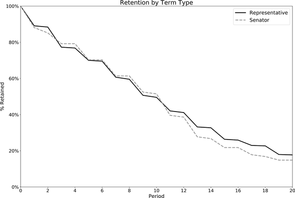
Figure 4-10. Retention by term type for legislators in office during the year 2000
A common use case for cohorting on a value other than a starting value is when trying to analyze retention after an entity has reached a threshold, such as a certain number of purchases or a certain amount spent. As with any cohort, it’s important to take care in defining what qualifies an entity to be in a cohort and which date will be used as the starting date.
Cohort retention is a powerful way to understand the behavior of entities in a time series data set. We’ve seen how to calculate retention with SQL and how to cohort based on the time series itself or on other tables, and from points in the middle of entity life span. We also looked at how to use functions and JOINs to adjust dates within time series and compensate for sparse cohorts. There are several types of analyses that are related to cohort retention: analysis, survivorship, returnship, and cumulative calculations, all of which build off of the SQL code that we’ve developed for retention. Let’s turn to them next.
Related Cohort Analyses
In the last section, we learned how to write SQL for cohort retention analysis. Retention captures whether an entity was in a time series data set on a specific date or window of time. In addition to presence on a specific date, analysis is often interested in questions of how long an entity lasted, whether an entity did multiple actions, and how many of those actions occurred. These can all be answered with code that is similar to retention and is well suited to just about any cohorting criteria you like. Let’s take a look at the first of these, survivorship.
Survivorship
Survivorship, also called survival analysis, is concerned with questions about how long something lasts, or the duration of time until a particular event such as churn or death. Survivorship analysis can answer questions about the share of the population that is likely to remain past a certain amount of time. Cohorts can help identify or at least provide hypotheses about which characteristics or circumstances increase or decrease the survival likelihood.
This is similar to a retention analysis, but instead of calculating whether an entity was present in a certain period, we calculate whether the entity is present in that period or later in the time series. Then the share of the total cohort is calculated. Typically one or more periods are chosen depending on the nature of the data set analyzed. For example, if we want to know the share of game players who survive for a week or longer, we can check for actions that occur after a week from starting and consider those players still surviving. On the other hand, if we are concerned about the number of students who are still in school after a certain number of years, we could look for the absence of a graduation event in a data set. The number of periods can be SELECTed either by calculating an average or typical life span or by choosing time periods that are meaningful to the organization or process analyzed, such as a month, year, or longer time period.
In this example, we’ll look at the share of legislators who survived in office for a decade or more after their first term started. Since we don’t need to know the specific dates of each term, we can start by calculating the first and last term_start dates, using min and max aggregations:
SELECT id_bioguide
,min(term_start) as first_term
,max(term_start) as last_term
FROM legislators_terms
GROUP BY 1
;

id_bioguide  first_term  last_term
-----------  ----------  ---------
A000118      1975-01-14  1977-01-04
P000281      1933-03-09  1937-01-05
K000039      1933-03-09  1951-01-03
...          ...         ...
Next, we add to the query a date_part function to find the century of the min term_start, and we calculate the tenure as the number of years between the min and max term_starts found with the age function:
SELECT id_bioguide
,date_part('century',min(term_start)) as first_century
,min(term_start) as first_term
,max(term_start) as last_term
,date_part('year',age(max(term_start),min(term_start))) as tenure
FROM legislators_terms
GROUP BY 1
;

id_bioguide  first_century  first_term  last_term  tenure
-----------  -------------  ----------  ---------  ------
A000118      20.0           1975-01-14  1977-01-04  1.0
P000281      20.0           1933-03-09  1937-01-05  3.0
K000039      20.0           1933-03-09  1951-01-03  17.0
...          ...            ...         ...         ...
Finally, we calculate the cohort_size with a count of all the legislators, as well as calculating the number who survived for at least 10 years by using a CASE statement and count aggregation. The percent who survived is found by dividing these two values:
SELECT first_century
,count(distinct id_bioguide) as cohort_size
,count(distinct case when tenure >= 10 then id_bioguide
                     end) as survived_10
,count(distinct case when tenure >= 10 then id_bioguide end)
 / count(distinct id_bioguide) as pct_survived_10
FROM
(
    SELECT id_bioguide
    ,date_part('century',min(term_start)) as first_century
    ,min(term_start) as first_term
    ,max(term_start) as last_term
    ,date_part('year',age(max(term_start),min(term_start))) as tenure
    FROM legislators_terms
    GROUP BY 1
) a
GROUP BY 1
;

century  cohort  survived_10  pct_survived_10
-------  ------  -----------  ---------------
18       368     83           0.2255
19       6299    892          0.1416
20       5091    1853         0.3640
21       760     119          0.1566
Since terms may or may not be consecutive, we can also calculate the share of legislators in each century who survived for five or more total terms. In the subquery, add a count to find the total number of terms per legislator. Then in the outer query, divide the number of legislators with five or more terms by the total cohort size:
SELECT first_century
,count(distinct id_bioguide) as cohort_size
,count(distinct case when total_terms >= 5 then id_bioguide end)
 as survived_5
,count(distinct case when total_terms >= 5 then id_bioguide end)
 / count(distinct id_bioguide) as pct_survived_5_terms
FROM
(
    SELECT id_bioguide
    ,date_part('century',min(term_start)) as first_century
    ,count(term_start) as total_terms
    FROM legislators_terms
    GROUP BY 1
) a
GROUP BY 1
;

century  cohort  survived_5  pct_survived_5_terms
-------  ------  ----------  --------------------
18       368     63          0.1712
19       6299    711         0.1129
20       5091    2153        0.4229
21       760     205         0.2697
Ten years or five terms is somewhat arbitrary. We can also calculate the survivorship for each number of years or periods and display the results in graph or table form. Here, we calculate the survivorship for each number of terms from 1 to 20. This is accomplished through a Cartesian JOIN to a subquery that contains those integers derived by the generate_series function:
SELECT a.first_century, b.terms
,count(distinct id_bioguide) as cohort
,count(distinct case when a.total_terms >= b.terms then id_bioguide
                     end) as cohort_survived
,count(distinct case when a.total_terms >= b.terms then id_bioguide
                     end)
 / count(distinct id_bioguide) as pct_survived
FROM
(
    SELECT id_bioguide
    ,date_part('century',min(term_start)) as first_century
    ,count(term_start) as total_terms
    FROM legislators_terms
    GROUP BY 1
) a
JOIN
(
    SELECT generate_series as terms
    FROM generate_series(1,20,1)
) b on 1 = 1
GROUP BY 1,2
;

century  terms  cohort  cohort_survived  pct_survived
-------  -----  ------  ---------------  ------------
18       1      368     368              1.0000
18       2      368     249              0.6766
18       3      368     153              0.4157
...      ...    ...     ...              ...
The results are graphed in Figure 4-11. Survivorship was highest in the 20th century, a result that agrees with results we saw previously in which retention was also highest in the 20th century.
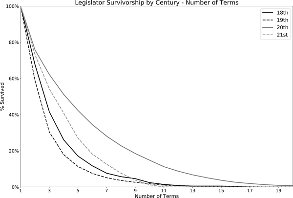
Figure 4-11. Survivorship for legislators: share of cohort who stayed in office for that many terms or longer
Survivorship is closely related to retention. While retention counts entities present in a specific number of periods from the start, survivorship considers only whether an entity was present as of a specific period or later. As a result, the code is simpler since it needs only the first and last dates in the time series, or a count of dates. Cohorting is done similar to cohorting for retention, and cohort definitions can come from within the time series or be derived from another table or subquery.
Next we’ll consider another type of analysis that is in some ways the inverse of survivorship. Rather than calculating whether an entity is present in the data set at a certain time or later, we will calculate whether an entity returns or repeats an action at a certain period or earlier. This is called returnship or repeat purchase behavior.
Returnship, or Repeat Purchase Behavior
Survivorship is useful for understanding how long a cohort is likely to stick around. Another useful type of cohort analysis seeks to understand whether a cohort member can be expected to return within a given window of time and the intensity of activity during that window. This is called returnship or repeat purchase behavior.
For example, an ecommerce site might want to know not only how many new buyers were acquired via a marketing campaign but also whether those buyers have become repeat buyers. One way to figure this out is to simply calculate total purchases per customer. However, comparing customers acquired two years ago with those acquired a month ago isn’t fair, since the former have had a much longer time in which to return. The older cohort would almost certainly appear more valuable than the newer one. Although this is true in a sense, it gives an incomplete picture of how the cohorts are likely to behave across their entire life span.
To make fair comparisons between cohorts with different starting dates, we need to create an analysis based on a time box, or a fixed window of time from the first date, and consider whether cohort members returned within that window. This way, every cohort has an equal amount of time under consideration, so long as we include only those cohorts for which the full window has elapsed. Returnship analysis is common for retail organizations, but it can also be applied in other domains. For example, a university might want to see how many students enrolled in a second course, or a hospital might be interested in how many patients need follow-up medical treatments after an initial incident.
To demonstrate returnship analysis, we can ask a new question of the legislators data set: how many legislators have more than one term type, and specifically, what share of them start as representatives and go on to become senators (some senators later become representatives, but that is much less common). Since relatively few make this transition, we’ll cohort legislators by the century in which they first became a representative.
The first step is to find the cohort size for each century, using the subquery and date_part calculations seen previously, for only those with term_type = 'rep':
SELECT date_part('century',a.first_term) as cohort_century
,count(id_bioguide) as reps
FROM
(
    SELECT id_bioguide, min(term_start) as first_term
    FROM legislators_terms
    WHERE term_type = 'rep'
    GROUP BY 1
) a
GROUP BY 1
;

cohort_century  reps
--------------  ----
18              299
19              5773
20              4481
21              683
Next we’ll perform a similar calculation, with a JOIN to the legislators_terms table, to find the representatives who later became senators. This is accomplished with the clauses b.term_type = 'sen' and b.term_start > a.first_term:
SELECT date_part('century',a.first_term) as cohort_century
,count(distinct a.id_bioguide) as rep_and_sen
FROM
(
    SELECT id_bioguide, min(term_start) as first_term
    FROM legislators_terms
    WHERE term_type = 'rep'
    GROUP BY 1
) a
JOIN legislators_terms b on a.id_bioguide = b.id_bioguide
and b.term_type = 'sen' and b.term_start > a.first_term
GROUP BY 1
;

cohort_century  rep_and_sen
--------------  -----------
18              57
19              329
20              254
21              25
Finally, we JOIN these two subqueries together and calculate the percent of representatives who became senators. A LEFT JOIN is used; this clause is typically recommended to ensure that all cohorts are included whether or not the subsequent event happened. If there is a century in which no representatives became senators, we still want to include that century in the result set:
SELECT aa.cohort_century
,bb.rep_and_sen / aa.reps as pct_rep_and_sen
FROM
(
    SELECT date_part('century',a.first_term) as cohort_century
    ,count(id_bioguide) as reps
    FROM
    (
        SELECT id_bioguide, min(term_start) as first_term
        FROM legislators_terms
        WHERE term_type = 'rep'
        GROUP BY 1
    ) a
    GROUP BY 1
) aa
LEFT JOIN
(
    SELECT date_part('century',b.first_term) as cohort_century
    ,count(distinct b.id_bioguide) as rep_and_sen
    FROM
    (
        SELECT id_bioguide, min(term_start) as first_term
        FROM legislators_terms
        WHERE term_type = 'rep'
        GROUP BY 1
    ) b
    JOIN legislators_terms c on b.id_bioguide = b.id_bioguide
    and c.term_type = 'sen' and c.term_start > b.first_term
    GROUP BY 1
) bb on aa.cohort_century = bb.cohort_century
;

cohort_century  pct_rep_and_sen
--------------  ---------------
18              0.1906
19              0.0570
20              0.0567
21              0.0366
Representatives from the 18th century were most likely to become senators. However, we have not yet applied a time box to ensure a fair comparison. While we can safely assume that all legislators who served in the 18th and 19th centuries are no longer living, many of those who were first elected in the 20th and 21st centuries are still in the middle of their careers. Adding the filter WHERE age(c.term_start, b.first_term) <= interval '10 years' to subquery bb creates a time box of 10 years. Note that the window can easily be made larger or smaller by changing the constant in the interval. An additional filter applied to subquery a, WHERE first_term <= '2009-12-31', excludes those who were less than 10 years into their careers when the data set was assembled:
SELECT aa.cohort_century
,bb.rep_and_sen * 100.0 / aa.reps as pct_10_yrs
FROM
(
    SELECT date_part('century',a.first_term)::int as cohort_century
    ,count(id_bioguide) as reps
    FROM
    (
        SELECT id_bioguide, min(term_start) as first_term
        FROM legislators_terms
        WHERE term_type = 'rep'
        GROUP BY 1
    ) a
    WHERE first_term <= '2009-12-31'
    GROUP BY 1
) aa
LEFT JOIN
(
    SELECT date_part('century',b.first_term)::int as cohort_century
    ,count(distinct b.id_bioguide) as rep_and_sen
    FROM
    (
        SELECT id_bioguide, min(term_start) as first_term
        FROM legislators_terms
        WHERE term_type = 'rep'
        GROUP BY 1
    ) b
    JOIN legislators_terms c on b.id_bioguide = c.id_bioguide
    and c.term_type = 'sen' and c.term_start > b.first_term
    WHERE age(c.term_start, b.first_term) <= interval '10 years'
    GROUP BY 1
) bb on aa.cohort_century = bb.cohort_century
;

Cohort_century  pct_10_yrs
--------------  ----------
18              0.0970
19              0.0244
20              0.0348
21              0.0764
With this new adjustment, the 18th century still had the highest share of representatives becoming senators within 10 years, but the 21st century has the second-highest share, and the 20th century had a higher share than the 19th.
Since 10 years is somewhat arbitrary, we might also want to compare several time windows. One option is to run the query several times with different intervals and note the results. Another option is to calculate multiple windows in the same result set by using a set of CASE statements inside of count distinct aggregations to form the intervals, rather than specifying the interval in the WHERE clause:
SELECT aa.cohort_century
,bb.rep_and_sen_5_yrs * 1.0 / aa.reps as pct_5_yrs
,bb.rep_and_sen_10_yrs * 1.0 / aa.reps as pct_10_yrs
,bb.rep_and_sen_15_yrs * 1.0 / aa.reps as pct_15_yrs
FROM
(
    SELECT date_part('century',a.first_term) as cohort_century
    ,count(id_bioguide) as reps
    FROM
    (
        SELECT id_bioguide, min(term_start) as first_term
        FROM legislators_terms
        WHERE term_type = 'rep'
        GROUP BY 1
    ) a
    WHERE first_term <= '2009-12-31'
    GROUP BY 1
) aa
LEFT JOIN
(
    SELECT date_part('century',b.first_term) as cohort_century
    ,count(distinct case when age(c.term_start,b.first_term)
                              <= interval '5 years'
                         then b.id_bioguide end) as rep_and_sen_5_yrs
    ,count(distinct case when age(c.term_start,b.first_term)
                              <= interval '10 years'
                         then b.id_bioguide end) as rep_and_sen_10_yrs
    ,count(distinct case when age(c.term_start,b.first_term)
                              <= interval '15 years'
                         then b.id_bioguide end) as rep_and_sen_15_yrs
    FROM
    (
        SELECT id_bioguide, min(term_start) as first_term
        FROM legislators_terms
        WHERE term_type = 'rep'
        GROUP BY 1
    ) b
    JOIN legislators_terms c on b.id_bioguide = c.id_bioguide
    and c.term_type = 'sen' and c.term_start > b.first_term
    GROUP BY 1
) bb on aa.cohort_century = bb.cohort_century
;

cohort_century  pct_5_yrs  pct_10_yrs  pct_15_yrs
--------------  ---------  ----------  ----------
18              0.0502     0.0970      0.1438
19              0.0088     0.0244      0.0409
20              0.0100     0.0348      0.0478
21              0.0400     0.0764      0.0873
With this output, we can see how the share of representatives who became senators evolved over time, both within each cohort and across cohorts. In addition to the table format, graphing the output often reveals interesting trends. In Figure 4-12, the cohorts based on century are replaced with cohorts based on the first decade, and the trends over 10 and 20 years are shown. Conversion of representatives to senators during the first few decades of the new US legislature was clearly different from patterns in the years since.
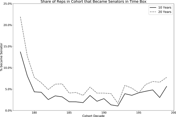
Figure 4-12. Trend of the share of representatives for each cohort, defined by starting decade, who later became senators
Finding the repeat behavior within a fixed time box is a useful tool for comparing cohorts. This is particularly true when the behaviors are intermittent in nature, such as purchase behavior or content or service consumption. In the next section, we’ll look at how to calculate not only whether an entity had a subsequent action but also how many subsequent actions they had, and we’ll aggregate them with cumulative calculations.
Cumulative Calculations
Cumulative cohort analysis can be used to establish cumulative lifetime value, also called customer lifetime value (the acronyms CLTV and LTV are used interchangeably), and to monitor newer cohorts in order to be able to predict what their full LTV will be. This is possible because early behavior is often highly correlated with long-term behavior. Users of a service who return frequently in their first days or weeks of using it tend to be the most likely to stay around over the long term. Customers who buy a second or third time early on are likely to continue purchasing over a longer time period. Subscribers who renew after the first month or year are often likely to stick around over many subsequent months or years.
In this section, I’ll mainly talk about the revenue-generating activities of customers, but this analysis can also be applied to situations in which customers or entities incur costs, such as through product returns, support interactions, or use of health-care services.
With cumulative calculations, we’re less concerned about whether an entity did an action on a particular date and more about the total as of a particular date. The cumulative calculations used in this type of analysis are most often counts or sums. We will again use the time box concept to ensure apples-to-apples comparisons between cohorts. Let’s look at the number of terms started within 10 years of the first term_start, cohorting the legislators by century and type of first term:
SELECT date_part('century',a.first_term) as century
,first_type
,count(distinct a.id_bioguide) as cohort
,count(b.term_start) as terms
FROM
(
    SELECT distinct id_bioguide
    ,first_value(term_type) over (partition by id_bioguide
                                  order by term_start) as first_type
    ,min(term_start) over (partition by id_bioguide) as first_term
    ,min(term_start) over (partition by id_bioguide)
     + interval '10 years' as first_plus_10
    FROM legislators_terms
) a
LEFT JOIN legislators_terms b on a.id_bioguide = b.id_bioguide
and b.term_start between a.first_term and a.first_plus_10
GROUP BY 1,2
;

century  first_type  cohort  terms
-------  ----------  ------  -----
18       rep         297     760
18       sen         71      101
19       rep         5744    12165
19       sen         555     795
20       rep         4473    16203
20       sen         618     1008
21       rep         683     2203
21       sen         77      118
The largest cohort is that of representatives first elected in the 19th century, but the cohort with the largest number of terms started within 10 years is that of representatives first elected in the 20th century. This type of calculation can be useful for understanding the overall contribution of a cohort to an organization. Total sales or total repeat purchases can be valuable metrics. Usually, though, we want to normalize to understand the contribution on a per-entity basis. Calculations we might want to make include average actions per person, average order value (AOV), items per order, and orders per customer. To normalize by the cohort size, simply divide by the starting cohort, which we’ve done previously with retention, survivorship, and returnship. Here we do that and also pivot the results into table form for easier comparisons:
SELECT century
,max(case when first_type = 'rep' then cohort end) as rep_cohort
,max(case when first_type = 'rep' then terms_per_leg end)
 as avg_rep_terms
,max(case when first_type = 'sen' then cohort end) as sen_cohort
,max(case when first_type = 'sen' then terms_per_leg end)
 as avg_sen_terms
FROM
(
    SELECT date_part('century',a.first_term) as century
    ,first_type
    ,count(distinct a.id_bioguide) as cohort
    ,count(b.term_start) as terms
    ,count(b.term_start)
     / count(distinct a.id_bioguide) as terms_per_leg
    FROM
    (
        SELECT distinct id_bioguide
        ,first_value(term_type) over (partition by id_bioguide
                                      order by term_start
                                      ) as first_type
        ,min(term_start) over (partition by id_bioguide) as first_term
        ,min(term_start) over (partition by id_bioguide)
         + interval '10 years' as first_plus_10
        FROM legislators_terms
    ) a
    LEFT JOIN legislators_terms b on a.id_bioguide = b.id_bioguide
    and b.term_start between a.first_term and a.first_plus_10
    GROUP BY 1,2
) aa
GROUP BY 1
;

century  rep_cohort  avg_rep_terms  sen_cohort  avg_sen_terms
-------  ----------  -------------  ----------  -------------
18       297         2.6            71          1.4
19       5744        2.1            555         1.4
20       4473        3.6            618         1.6
21       683         3.2            77          1.5
With the cumulative terms normalized by the cohort size, we can now confirm that representatives first elected in the 20th century had the highest average number of terms, while those who started in the 19th century had the fewest number of terms on average. Senators have fewer but longer terms than their representative peers, and again those who started in the 20th century have had the highest number of terms on average.
Cumulative calculations are often used in customer lifetime value calculations. LTV is usually calculated using monetary measures, such as total dollars spent by a customer, or the gross margin (revenue minus costs) generated by a customer across their lifetime. To facilitate comparisons between cohorts, the “lifetime” is often chosen to reflect average customer lifetime, or periods that are convenient to analyze, such as 3, 5, or 10 years. The legislators data set doesn’t contain financial metrics, but swapping in dollar values in any of the preceding SQL code would be straightforward. Fortunately, SQL is a flexible enough language that we can adapt these templates to address a wide variety of analytical questions.
Cohort analysis includes a set of techniques that can be used to answer questions related to behavior over time and how various attributes may contribute to differences between groups. Survivorship, returnship, and cumulative calculations all shed light on these questions. With a good understanding of how cohorts behave, we often have to turn our attention back to the composition or mix of cohorts over time, understanding how that can impact total retention, survivorship, returnship, or cumulative values such that these measures differ surprisingly from the individual cohorts.
Cross-Section Analysis, Through a Cohort Lens
So far in this chapter, we’ve been looking at cohort analysis. We’ve followed the behavior of cohorts across time with retention, survivorship, returnship, and cumulative behavior analyses. One of the challenges with these analyses, however, is that even as they make changes within cohorts easy to spot, it can be difficult to spot changes in the overall composition of a customer or user base.
Mix shifts, which are changes in the composition of the customer or user base over time, can also occur, making later cohorts different from earlier ones. Mix shifts may be due to international expansion, shifting between organic and paid acquisition strategies, or moving from a niche enthusiast audience to a broader mass market one. Creating additional cohorts, or segments, along any of these suspected lines can help diagnose whether a mix shift is happening.
Cohort analysis can be contrasted with cross-sectional analysis, which compares individuals or groups at a single point in time. Cross-sectional studies can correlate years of education with current income, for example. On the positive side, collecting data sets for cross-sectional analysis is often easier since no time series is necessary. Cross-sectional analysis can be insightful, generating hypotheses for further investigation. On the negative side, a form of selection bias called survivorship bias usually exists, which can lead to false conclusions.
Cohort analysis is a way to overcome survivorship bias by including all members of a starting cohort in the analysis. We can take a series of cross sections from a cohort analysis to understand how the mix of entities may have changed over time. On any given date, users from a variety of cohorts are present. We can use cross-sectional analysis to examine them, like layers of sediment, to reveal new insights. In the next example, we’ll create a time series of the share of legislators from each cohort for each year in the data set.
The first step is to find the number of legislators in office each year by JOINing the legislators table to the date_dim, WHERE the date from the date_dim is between the start and end dates of each term. Here we use December 31 for each year to find the legislators in office at each year’s end:
SELECT b.date, count(distinct a.id_bioguide) as legislators
FROM legislators_terms a
JOIN date_dim b on b.date between a.term_start and a.term_end
and b.month_name = 'December' and b.day_of_month = 31
and b.year <= 2019
GROUP BY 1
;

date        legislators
----------  -----------
1789-12-31  89
1790-12-31  95
1791-12-31  99
...         ...
Next, we add in the century cohorting criteria by JOINing to a subquery with the first_term calculated:
SELECT b.date
,date_part('century',first_term) as century
,count(distinct a.id_bioguide) as legislators
FROM legislators_terms a
JOIN date_dim b on b.date between a.term_start and a.term_end
 and b.month_name = 'December' and b.day_of_month = 31
 and b.year <= 2019
JOIN
(
    SELECT id_bioguide, min(term_start) as first_term
    FROM legislators_terms
    GROUP BY 1
) c on a.id_bioguide = c.id_bioguide
GROUP BY 1,2
;

date        century  legislators
----------  -------  -----------
1789-12-31  18       89
1790-12-31  18       95
1791-12-31  18       99
...         ...      ...
Finally, we calculate the percent of total legislators in each year that the century cohort represents. This can be done in a couple of ways, depending on the shape of output desired. The first way is to keep a row for each date and century combination and use a sum window function in the denominator of the percentage calculation:
SELECT date
,century
,legislators
,sum(legislators) over (partition by date) as cohort
,legislators / sum(legislators) over (partition by date)
 as pct_century
FROM
(
    SELECT b.date
    ,date_part('century',first_term) as century
    ,count(distinct a.id_bioguide) as legislators
    FROM legislators_terms a
    JOIN date_dim b on b.date between a.term_start and a.term_end
    and b.month_name = 'December' and b.day_of_month = 31
    and b.year <= 2019
    JOIN
    (
        SELECT id_bioguide, min(term_start) as first_term
        FROM legislators_terms
        GROUP BY 1
    ) c on a.id_bioguide = c.id_bioguide
    GROUP BY 1,2
) a
;

date        century  legislators  cohort  pct_century
----------  -------  -----------  ------  -----------
2018-12-31  20       122          539     0.2263
2018-12-31  21       417          539     0.7737
2019-12-31  20       97           537     0.1806
2019-12-31  21       440          537     0.8194
...         ...      ...          ...     ...
The second approach results in one row per year, with a column for each century, a table format that may be easier to scan for trends:
SELECT date
,coalesce(sum(case when century = 18 then legislators end)
          / sum(legislators),0) as pct_18
,coalesce(sum(case when century = 19 then legislators end)
          / sum(legislators),0) as pct_19
,coalesce(sum(case when century = 20 then legislators end)
          / sum(legislators),0) as pct_20
,coalesce(sum(case when century = 21 then legislators end)
          / sum(legislators),0) as pct_21
FROM
(
    SELECT b.date
    ,date_part('century',first_term) as century
    ,count(distinct a.id_bioguide) as legislators
    FROM legislators_terms a
    JOIN date_dim b on b.date between a.term_start and a.term_end
     and b.month_name = 'December' and b.day_of_month = 31
     and b.year <= 2019
    JOIN
    (
        SELECT id_bioguide, min(term_start) as first_term
        FROM legislators_terms
        GROUP BY 1
    ) c on a.id_bioguide = c.id_bioguide
    GROUP BY 1,2
) aa
GROUP BY 1
;


date        pct_18  pct_19  pct_20  pct_21
----------  ------  ------  ------  ------
2017-12-31  0       0       0.2305  0.7695
2018-12-31  0       0       0.2263  0.7737
2019-12-31  0       0       0.1806  0.8193
...         ...     ...     ...     ...
We can graph the output, as in Figure 4-13, to see how newer cohorts of legislators gradually overtake older cohorts, until they themselves are replaced by new cohorts.
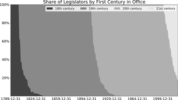
Figure 4-13. Percent of legislators each year, by century first elected
Rather than cohorting on first_term, we can cohort on tenure instead. Finding the share of customers who are relatively new, are of medium tenure, or are long-term customers at various points in time can be insightful. Let’s take a look at how the tenure of legislators in Congress has changed over time.
The first step is to calculate, for each year, the cumulative number of years in office for each legislator. Since there can be gaps between terms when legislators are voted out or leave office for other reasons, we’ll first find each year in which the legislator was in office at the end of the year, in the subquery. Then we’ll use a count window function, with the window covering the rows unbounded preceding, or all prior rows for that legislator, and current row:
SELECT id_bioguide, date
,count(date) over (partition by id_bioguide
                   order by date rows between
                   unbounded preceding and current row
                   ) as cume_years
FROM
(
    SELECT distinct a.id_bioguide, b.date
    FROM legislators_terms a
    JOIN date_dim b on b.date between a.term_start and a.term_end
     and b.month_name = 'December' and b.day_of_month = 31
     and b.year <= 2019
) aa
;

id_bioguide  date        cume_years
-----------  ----------  ----------
A000001      1951-12-31  1
A000001      1952-12-31  2
A000002      1947-12-31  1
A000002      1948-12-31  2
A000002      1949-12-31  3
...          ...         ...
Next, count the number of legislators for each combination of date and cume_years to create a distribution:
SELECT date, cume_years
,count(distinct id_bioguide) as legislators
FROM
(
SELECT id_bioguide, date
,count(date) over (partition by id_bioguide
                   order by date rows between
                   unbounded preceding and current row
                   ) as cume_years
FROM
(
    SELECT distinct a.id_bioguide, b.date
    FROM legislators_terms a
    JOIN date_dim b on b.date between a.term_start and a.term_end
     and b.month_name = 'December' and b.day_of_month = 31
     and b.year <= 2019
    GROUP BY 1,2
    ) aa
) aaa
GROUP BY 1,2
;

date         cume_years  legislators
-----------  ----------  ----------
1789-12-31   1           89
1790-12-31   1           6
1790-12-31   2           89
1791-12-31   1           37
...          ...         ...
Before calculating the percentage for each tenure per year and adjusting the presentation format, we might want to consider grouping the tenures. A quick profiling of our results so far reveals that in some years, almost 40 different tenures are represented. This will likely be difficult to visualize and interpret:
SELECT date, count(*) as tenures
FROM
(
    SELECT date, cume_years
    ,count(distinct id_bioguide) as legislators
    FROM
    (
        SELECT id_bioguide, date
        ,count(date) over (partition by id_bioguide
                           order by date rows between
                           unbounded preceding and current row
                           ) as cume_years
        FROM
        (
            SELECT distinct a.id_bioguide, b.date
            FROM legislators_terms a
            JOIN date_dim b
             on b.date between a.term_start and a.term_end
             and b.month_name = 'December' and b.day_of_month = 31
             and b.year <= 2019
            GROUP BY 1,2
        ) aa
    ) aaa
    GROUP BY 1,2
) aaaa
GROUP BY 1
;

date         tenures
-----------  -------
1998-12-31   39
1994-12-31   39
1996-12-31   38
...          ...
As a result, we may want to group the values. There is no single right way to group tenures. If there are organizational definitions of tenure groups, go ahead and use them. Otherwise, I usually try to break them up into three to five groups of roughly equal size. Here we’ll group the tenures into four cohorts, where cume_years is less than or equal to 4 years, between 5 and 10 years, between 11 and 20 years, and equal to or more than 21 years:
SELECT date, tenure
,legislators / sum(legislators) over (partition by date)
 as pct_legislators
FROM
(
    SELECT date
    ,case when cume_years <= 4 then '1 to 4'
          when cume_years <= 10 then '5 to 10'
          when cume_years <= 20 then '11 to 20'
          else '21+' end as tenure
    ,count(distinct id_bioguide) as legislators
    FROM
    (
        SELECT id_bioguide, date
        ,count(date) over (partition by id_bioguide
                           order by date rows between
                           unbounded preceding and current row
                           ) as cume_years
        FROM
        (
            SELECT distinct a.id_bioguide, b.date
            FROM legislators_terms a
            JOIN date_dim b
             on b.date between a.term_start and a.term_end
             and b.month_name = 'December' and b.day_of_month = 31
             and b.year <= 2019
            GROUP BY 1,2
        ) a
    ) aa
    GROUP BY 1,2
) aaa
;

date        tenure    pct_legislators
----------  -------   ---------------
2019-12-31  1 to 4    0.2998
2019-12-31  5 to 10   0.3203
2019-12-31  11 to 20  0.2011
2019-12-31  21+       0.1788
...         ...       ...
The graphing of the results in Figure 4-14 shows that in the early years of the country, most legislators had very little tenure. In more recent years, the share of legislators with 21 or more years in office has been increasing. There are also interesting periodic increases in 1-to-4-year-tenure legislators that may reflect shifts in political trends.
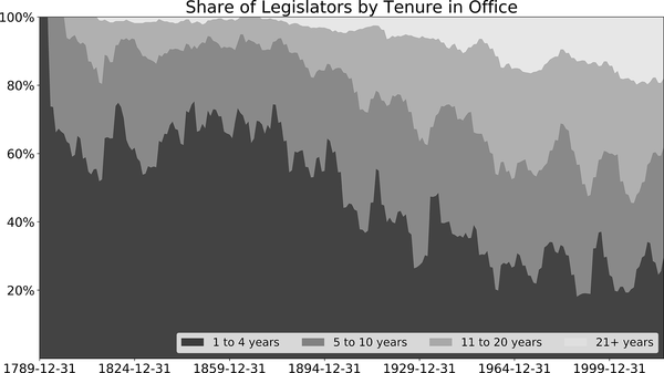
Figure 4-14. Percent of legislators by number of years in office
A cross section of a population at any point in time is made up of members from multiple cohorts. Creating a time series of these cross sections is another interesting way of analyzing trends. Combining this with insights from retention can provide a more robust picture of trends in any organization.
Conclusion
Cohort analysis is a useful way to investigate how groups change over time, whether it be from the perspective of retention, repeat behavior, or cumulative actions. Cohort analysis is retrospective, looking back at populations using intrinsic attributes or attributes derived from behavior. Interesting and hopefully useful correlations can be found through this type of analysis. However, as the saying goes, correlation does not imply causation. To determine actual causality, randomized experiments are the gold standard. Chapter 7 will go into depth on experiment analysis.
Before we turn to experimentation, however, we have a few other types of analysis to cover. Next we’ll cover text analysis: components of text analysis often show up in other analyses, and it’s an interesting facet of analysis in itself.
Get SQL for Data Analysis now with the O’Reilly learning platform.
O’Reilly members experience books, live events, courses curated by job role, and more from O’Reilly and nearly 200 top publishers.

