SQL for Data Analysis

Chapter 1. Analysis with SQL

If you’re reading this book, you’re probably interested in data analysis and in using SQL to accomplish it. You may be experienced with data analysis but new to SQL, or perhaps you’re experienced with SQL but new to data analysis. Or you may be new to both topics entirely. Whatever your starting point, this chapter lays the groundwork for the topics covered in the rest of the book and makes sure we have a common vocabulary. I’ll start with a discussion of what data analysis is and then move on to a discussion of SQL: what it is, why it’s so popular, how it compares to other tools, and how it fits into data analysis. Then, since modern data analysis is so intertwined with the technologies that have enabled it, I’ll conclude with a discussion of different types of databases that you may encounter in your work, why they’re used, and what all of that means for the SQL you write.

What Is Data Analysis?

Collecting and storing data for analysis is a very human activity. Systems to track stores of grain, taxes, and the population go back thousands of years, and the roots of statistics date back hundreds of years. Related disciplines, including statistical process control, operations research, and cybernetics, exploded in the 20th century. Many different names are used to describe the discipline of data analysis, such as business intelligence (BI), analytics, data science, and decision science, and practitioners have a range of job titles. Data analysis is also done by marketers, product managers, business analysts, and a variety of other people. In this book, I’ll use the terms data analyst and data scientist interchangeably to mean the person working with SQL to understand data. I will refer to the software used to build reports and dashboards as BI tools.

Data analysis in the contemporary sense was enabled by, and is intertwined with, the history of computing. Trends in both research and commercialization have shaped it, and the story includes a who’s who of researchers and major companies, which we’ll talk about in the section on SQL. Data analysis blends the power of computing with techniques from traditional statistics. Data analysis is part data discovery, part data interpretation, and part data communication. Very often the purpose of data analysis is to improve decision making, by humans and increasingly by machines through automation.

Sound methodology is critical, but analysis is about more than just producing the right number. It’s about curiosity, asking questions, and the “why” behind the numbers. It’s about patterns and anomalies, discovering and interpreting clues about how businesses and humans behave. Sometimes analysis is done on a data set gathered to answer a specific question, as in a scientific setting or an online experiment. Analysis is also done on data that is generated as a result of doing business, as in sales of a company’s products, or that is generated for analytics purposes, such as user interaction tracking on websites and mobile apps. This data has a wide range of possible applications, from troubleshooting to planning user interface (UI) improvements, but it often arrives in a format and volume such that the data needs processing before yielding answers. Chapter 2 will cover preparing data for analysis, and Chapter 8 will discuss some of the ethical and privacy concerns with which all data practitioners should be familiar.

It’s hard to think of an industry that hasn’t been touched by data analysis: manufacturing, retail, finance, health care, education, and even government have all been changed by it. Sports teams have employed data analysis since the early years of Billy Beane’s term as general manager of the Oakland Athletics, made famous by Michael Lewis’s book Moneyball (Norton). Data analysis is used in marketing, sales, logistics, product development, user experience design, support centers, human resources, and more. The combination of techniques, applications, and computing power has led to the explosion of related fields such as data engineering and data science.

Data analysis is by definition done on historical data, and it’s important to remember that the past doesn’t necessarily predict the future. The world is dynamic, and organizations are dynamic as well—new products and processes are introduced, competitors rise and fall, sociopolitical climates change. Criticisms are leveled against data analysis for being backward looking. Though that characterization is true, I have seen organizations gain tremendous value from analyzing historical data. Mining historical data helps us understand the characteristics and behavior of customers, suppliers, and processes. Historical data can help us develop informed estimates and predicted ranges of outcomes, which will sometimes be wrong but quite often will be right. Past data can point out gaps, weaknesses, and opportunities. It allows organizations to optimize, save money, and reduce risk and fraud. It can also help organizations find opportunity, and it can become the building blocks of new products that delight customers.

Note

Organizations that don’t do some form of data analysis are few and far between these days, but there are still some holdouts. Why do some organizations not use data analysis? One argument is the cost-to-value ratio. Collecting, processing, and analyzing data takes work and some level of financial investment. Some organizations are too new, or they’re too haphazard. If there isn’t a consistent process, it’s hard to generate data that’s consistent enough to analyze. Finally, there are ethical considerations. Collecting or storing data about certain people in certain situations may be regulated or even banned. Data about children and health-care interventions is sensitive, for example, and there are extensive regulations around its collection. Even organizations that are otherwise data driven need to take care around customer privacy and to think hard about what data should be collected, why it is needed, and how long it should be stored. Regulations such as the European Union’s General Data Protection Regulation, or GDPR, and the California Consumer Privacy Act, or CCPA, have changed the way businesses think about consumer data. We’ll discuss these regulations in more depth in Chapter 8. As data practitioners, we should always be thinking about the ethical implications of our work.

When working with organizations, I like to tell people that data analysis is not a project that wraps up at a fixed date—it’s a way of life. Developing a data-informed mindset is a process, and reaping the rewards is a journey. Unknowns become known, difficult questions are chipped away at until there are answers, and the most critical information is embedded in dashboards that power tactical and strategic decisions. With this information, new and harder questions are asked, and then the process repeats.

Data analysis is both accessible for those looking to get started and hard to master. The technology can be learned, particularly SQL. Many problems, such as optimizing marketing spend or detecting fraud, are familiar and translate across businesses. Every organization is different and every data set has quirks, so even familiar problems can pose new challenges. Communicating results is a skill. Learning to make good recommendations and becoming a trusted partner to an organization take time. In my experience, simple analysis presented persuasively has more impact than sophisticated analysis presented poorly. Successful data analysis also requires partnership. You can have great insights, but if there is no one to execute on them, you haven’t really made an impact. Even with all the technology, it’s still about people, and relationships matter.

Why SQL?

This section describes what SQL is, the benefits of using it, how it compares to other languages commonly used for analysis, and finally how SQL fits into the analysis workflow.

What Is SQL?

SQL is the language used to communicate with databases. The acronym stands for Structured Query Language and is pronounced either like “sequel” or by saying each letter, as in “ess cue el.” This is only the first of many controversies and inconsistencies surrounding SQL that we’ll see, but most people will know what you mean regardless of how you say it. There is some debate as to whether SQL is or isn’t a programming language. It isn’t a general purpose language in the way that C or Python are. SQL without a database and data in tables is just a text file. SQL can’t build a website, but it is powerful for working with data in databases. On a practical level, what matters most is that SQL can help you get the job of data analysis done.

IBM was the first to develop SQL databases, from the relational model invented by Edgar Codd in the 1960s. The relational model was a theoretical description for managing data using relationships. By creating the first databases, IBM helped to advance the theory, but it also had commercial considerations, as did Oracle, Microsoft, and every other company that has commercialized a database since. From the beginning, there has been tension between computer theory and commercial reality. SQL became an International Organization for Standards (ISO) standard in 1987 and an American National Standards Institute (ANSI) standard in 1986. Although all major databases start from these standards in their implementation of SQL, many have variations and functions that make life easier for the users of those databases. These come at the cost of making SQL more difficult to move between databases without some modifications.

SQL is used to access, manipulate, and retrieve data from objects in a database. Databases can have one or more schemas, which provide the organization and structure and contain other objects. Within a schema, the objects most commonly used in data analysis are tables, views, and functions. Tables contain fields, which hold the data. Tables may have one or more indexes; an index is a special kind of data structure that allows data to be retrieved more efficiently. Indexes are usually defined by a database administrator. Views are essentially stored queries that can be referenced in the same way as a table. Functions allow commonly used sets of calculations or procedures to be stored and easily referenced in queries. They are usually created by a database administrator, or DBA. Figure 1-1 gives an overview of the organization of databases.

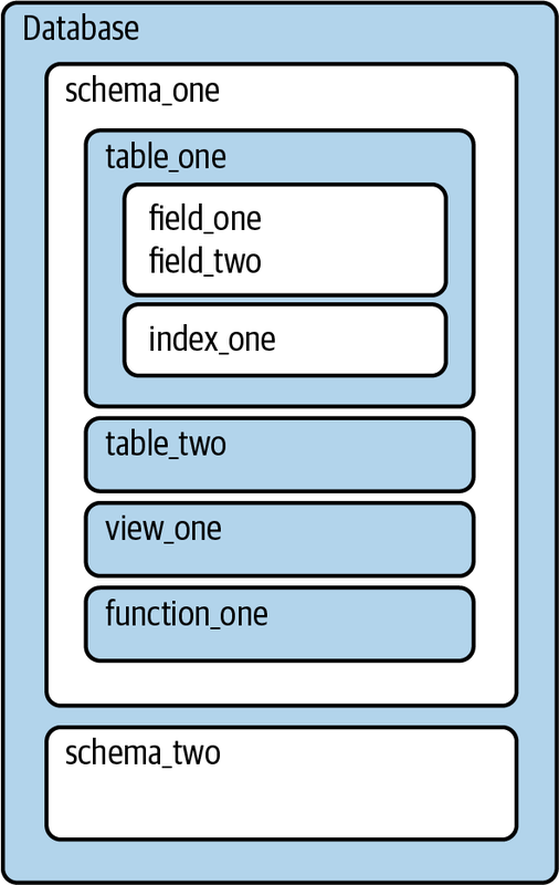
Figure 1-1. Overview of database organization and objects in a database

To communicate with databases, SQL has four sublanguages for tackling different jobs, and these are mostly standard across database types. Most people who work in data analysis don’t need to recall the names of these sublanguages on a daily basis, but they might come up in conversation with database administrators or data engineers, so I’ll briefly introduce them. The commands all work fluidly together, and some may coexist in the same SQL statement.

DQL, or data query language, is what this book is mainly about. It’s used for querying data, which you can think of as using code to ask questions of a database. DQL commands include SELECT, which will be familiar to prior users of SQL, but the acronym DQL is not frequently used in my experience. SQL queries can be as short as a single line or span many tens of lines. SQL queries can access a single table (or view), can combine data from multiple tables through the use of joins, and can also query across multiple schemas in the same database. SQL queries generally cannot query across databases, but in some cases clever network settings or additional software can be used to retrieve data from multiple sources, even databases of different types. SQL queries are self-contained and, apart from tables, do not reference variables or outputs from previous steps not contained in the query, unlike scripting languages.

DDL, or data definition language, is used to create and modify tables, views, users, and other objects in the database. It affects the structure but not the contents. There are three common commands: CREATE, ALTER, and DROP. CREATE is used to make new objects. ALTER changes the structure of an object, such as by adding a column to a table. DROP deletes the entire object and its structure. You might hear DBAs and data engineers talk about working with DDLs—this is really just shorthand for the files or pieces of code that do the creates, alters, or drops. An example of how DDL is used in the context of analysis is the code to create temporary tables.

DCL, or data control language, is used for access control. Commands include GRANT and REVOKE, which give permission and remove permission, respectively. In an analysis context, GRANT might be needed to allow a colleague to query a table you created. You might also encounter such a command when someone has told you a table exists in the database but you can’t see it—permissions might need to be GRANTed to your user.

DML, or data manipulation language, is used to act on the data itself. The commands are INSERT, UPDATE, and DELETE. INSERT adds new records and is essentially the “load” step in extract, transform, load (ETL). UPDATE changes values in a field, and DELETE removes rows. You will encounter these commands if you have any kind of self-managed tables—temp tables, sandbox tables—or if you find yourself in the role of both owner and analyzer of the database.

These four sublanguages are present in all major databases. In this book, I’ll focus mainly on DQL. We will touch on a few DDL and DML commands in Chapter 8, and you will also see some examples in the GitHub site for the book, where they are used to create and populate the data used in examples. Thanks to this common set of commands, SQL code written for any database will look familiar to anyone used to working with SQL. However, reading SQL from another database may feel a bit like listening to someone who speaks the same language as you but comes from another part of the country or the world. The basic structure of the language is the same, but the slang is different, and some words have different meanings altogether. Variations in SQL from database to database are often termed dialects, and database users will reference Oracle SQL, MSSQL, or other dialects.

Still, once you know SQL, you can work with different database types as long as you pay attention to details such as the handling of nulls, dates, and timestamps; the division of integers; and case sensitivity.

This book uses PostgreSQL, or Postgres, for the examples, though I will try to point out where the code would be meaningfully different in other types of databases. You can install Postgres on a personal computer in order to follow along with the examples.

Benefits of SQL

There are many good reasons to use SQL for data analysis, from computing power to its ubiquity in data analysis tools and its flexibility.

Perhaps the best reason to use SQL is that much of the world’s data is already in databases. It’s likely your own organization has one or more databases. Even if data is not already in a database, loading it into one can be worthwhile in order to take advantage of the storage and computing advantages, especially when compared to alternatives such as spreadsheets. Computing power has exploded in recent years, and data warehouses and data infrastructure have evolved to take advantage of it. Some newer cloud databases allow massive amounts of data to be queried in memory, speeding things up further. The days of waiting minutes or hours for query results to return may be over, though analysts may just write more complex queries in response.

SQL is the de facto standard for interacting with databases and retrieving data from them. A wide range of popular software connects to databases with SQL, from spreadsheets to BI and visualization tools and coding languages such as Python and R (discussed in the next section). Due to the computing resources available, performing as much data manipulation and aggregation as possible in the database often has advantages downstream. We’ll discuss strategies for building complex data sets for downstream tools in depth in Chapter 8.

The basic SQL building blocks can be combined in an endless number of ways. Starting with a relatively small number of building blocks—the syntax—SQL can accomplish a wide array of tasks. SQL can be developed iteratively, and it’s easy to review the results as you go. It may not be a full-fledged programming language, but it can do a lot, from transforming data to performing complex calculations and answering questions.

Last, SQL is relatively easy to learn, with a finite amount of syntax. You can learn the basic keywords and structure quickly and then hone your craft over time working with varied data sets. Applications of SQL are virtually infinite, when you take into account the range of data sets in the world and the possible questions that can be asked of data. SQL is taught in many universities, and many people pick up some skills on the job. Even employees who don’t already have SQL skills can be trained, and the learning curve may be easier than that for other programming languages. This makes storing data for analysis in relational databases a logical choice for organizations.

SQL Versus R or Python

While SQL is a popular language for data analysis, it isn’t the only choice. R and Python are among the most popular of the other languages used for data analysis. R is a statistical and graphing language, while Python is a general-purpose programming language that has strengths in working with data. Both are open source, can be installed on a laptop, and have active communities developing packages, or extensions, that tackle various data manipulation and analysis tasks. Choosing between R and Python is beyond the scope of this book, but there are many discussions online about the relative advantages of each. Here I will consider them together as coding-language alternatives to SQL.

One major difference between SQL and other coding languages is where the code runs and, therefore, how much computing power is available. SQL always runs on a database server, taking advantage of all its computing resources. For doing analysis, R and Python are usually run locally on your machine, so computing resources are capped by whatever is available locally. There are, of course, lots of exceptions: databases can run on laptops, and R and Python can be run on servers with more resources. When you are performing anything other than the simplest analysis on large data sets, pushing work onto a database server with more resources is a good option. Since databases are usually set up to continually receive new data, SQL is also a good choice when a report or dashboard needs to update periodically.

A second difference is in how data is stored and organized. Relational databases always organize data into rows and columns within tables, so SQL assumes this structure for every query. R and Python have a wider variety of ways to store data, including variables, lists, and dictionaries, among other options. These provide more flexibility, but at the cost of a steeper learning curve. To facilitate data analysis, R has data frames, which are similar to database tables and organize data into rows and columns. The pandas package makes DataFrames available in Python. Even when other options are available, the table structure remains valuable for analysis.

Looping is another major difference between SQL and most other computer programming languages. A loop is an instruction or a set of instructions that repeats until a specified condition is met. SQL aggregations implicitly loop over the set of data, without any additional code. We will see later how the lack of ability to loop over fields can result in lengthy SQL statements when pivoting or unpivoting data. While deeper discussion is beyond the scope of this book, some vendors have created extensions to SQL, such as PL/SQL in Oracle and T-SQL in Microsoft SQL Server, that allow functionality such as looping.

A drawback of SQL is that your data must be in a database,¹ whereas R and Python can import data from files stored locally or can access files stored on servers or websites. This is convenient for many one-off projects. A database can be installed on a laptop, but this does add an extra layer of overhead. In the other direction, packages such as dbplyr for R and SQLAlchemy for Python allow programs written in those languages to connect to databases, execute SQL queries, and use the results in further processing steps. In this sense, R or Python can be complementary to SQL.

R and Python both have sophisticated statistical functions that are either built in or available in packages. Although SQL has, for example, functions to calculate average and standard deviation, calculations of p-values and statistical significance that are needed in experiment analysis (discussed in Chapter 7) cannot be performed with SQL alone. In addition to sophisticated statistics, machine learning is another area that is better tackled with one of these other coding languages.

When deciding whether to use SQL, R, or Python for an analysis, consider:

• Where is the data located—in a database, a file, a website?

• What is the volume of data?

• Where is the data going—into a report, a visualization, a statistical analysis?

• Will it need to be updated or refreshed with new data? How often?

• What does your team or organization use, and how important is it to conform to existing standards?

There is no shortage of debate around which languages and tools are best for doing data analysis or data science. As with many things, there’s often more than one way to accomplish an analysis. Programming languages evolve and change in popularity, and we’re lucky to live and work in a time with so many good choices. SQL has been around for a long time and will likely remain popular for years to come. The ultimate goal is to use the best available tool for the job. This book will help you get the most out of SQL for data analysis, regardless of what else is in your toolkit.

SQL as Part of the Data Analysis Workflow

Now that I’ve explained what SQL is, discussed some of its benefits, and compared it to other languages, we’ll turn to a discussion of where SQL fits in the data analysis process. Analysis work always starts with a question, which may be about how many new customers have been acquired, how sales are trending, or why some users stick around for a long time while others try a service and never return. Once the question is framed, we consider where the data originated, where the data is stored, the analysis plan, and how the results will be presented to the audience. Figure 1-2 shows the steps in the process. Queries and analysis are the focus of this book, though I will discuss the other steps briefly in order to put the queries and analysis stage into a broader context.

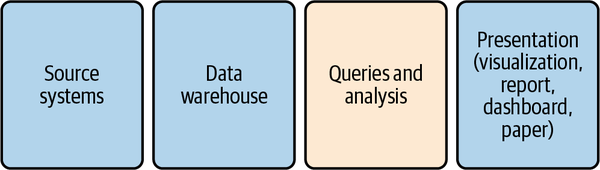
Figure 1-2. Steps in the data analysis process

First, data is generated by source systems, a term that includes any human or machine process that generates data of interest. Data can be generated by people by hand, such as when someone fills out a form or takes notes during a doctor’s visit. Data can also be machine generated, such as when an application database records a purchase, an event-streaming system records a website click, or a marketing management tool records an email open. Source systems can generate many different types and formats of data, and Chapter 2 will discuss them, and how the type of source may impact the analysis, in more detail.

The second step is moving the data and storing it in a database for analysis. I will use the terms data warehouse, which is a database that consolidates data from across an organization into a central repository, and data store, which refers to any type of data storage system that can be queried. Other terms you might come across are data mart, which is typically a subset of a data warehouse, or a more narrowly focused data warehouse; and data lake, a term that can mean either that data resides in a file storage system or that it is stored in a database but without the degree of data transformation that is common in data warehouses. Data warehouses range from small and simple to huge and expensive. A database running on a laptop will be sufficient for you to follow along with the examples in this book. What matters is having the data you need to perform an analysis together in one place.

Note

Usually a person or team is responsible for getting data into the data warehouse. This process is called ETL, or extract, transform, load. Extract pulls the data from the source system. Transform optionally changes the structure of the data, performs data quality cleaning, or aggregates the data. Load puts the data into the database. This process can also be called ELT, for extract, load, transform—the difference being that, rather than transformations being done before data is loaded, all the data is loaded and then transformations are performed, usually using SQL. You might also hear the terms source and target in the context of ETL. The source is where the data comes from, and the target is the destination, i.e., the database and the tables within it. Even when SQL is used to do the transforming, another language such as Python or Java is used to glue the steps together, coordinate scheduling, and raise alerts when something goes wrong. There are a number of commercial products as well as open source tools available, so teams don’t have to create an ETL system entirely from scratch.

Once the data is in a database, the next step is performing queries and analysis. In this step, SQL is applied to explore, profile, clean, shape, and analyze the data. Figure 1-3 shows the general flow of the process. Exploring the data involves becoming familiar with the topic, where the data was generated, and the database tables in which it is stored. Profiling involves checking the unique values and distribution of records in the data set. Cleaning involves fixing incorrect or incomplete data, adding categorization and flags, and handling null values. Shaping is the process of arranging the data into the rows and columns needed in the result set. Finally, analyzing the data involves reviewing the output for trends, conclusions, and insights. Although this process is shown as linear, in practice it is often cyclical—for example, when shaping or analysis reveals data that should be cleaned.

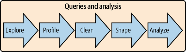
Figure 1-3. Stages within the queries and analysis step of the analysis workflow

Presentation of the data into a final output form is the last step in the overall workflow. Businesspeople won’t appreciate receiving a file of SQL code; they expect you to present graphs, charts, and insights. Communication is key to having an impact with analysis, and for that we need a way to share the results with other people. At other times, you may need to apply more sophisticated statistical analysis than is possible in SQL, or you may want to feed the data into a machine learning (ML) algorithm. Fortunately, most reporting and visualization tools have SQL connectors that allow you to pull in data from entire tables or prewritten SQL queries. Statistical software and languages commonly used for ML also usually have SQL connectors.

Analysis workflows encompass a number of steps and often include multiple tools and technologies. SQL queries and analysis are at the heart of many analyses and are what we will focus on in the following chapters. Chapter 2 will discuss types of source systems and the types of data they generate. The rest of this chapter will take a look at the types of databases you are likely to encounter in your analysis journey.

Database Types and How to Work with Them

If you’re working with SQL, you’ll be working with databases. There is a range of database types—open source to proprietary, row-store to column-store. There are on-premises databases and cloud databases, as well as hybrid databases, where an organization runs the database software on a cloud vendor’s infrastructure. There are also a number of data stores that aren’t databases at all but can be queried with SQL.

Databases are not all created equal; each database type has its strengths and weaknesses when it comes to analysis work. Unlike tools used in other parts of the analysis workflow, you may not have much say in which database technology is used in your organization. Knowing the ins and outs of the database you have will help you work more efficiently and take advantage of any special SQL functions it offers. Familiarity with other types of databases will help you if you find yourself working on a project to build or migrate to a new data warehouse. You may want to install a database on your laptop for personal, small-scale projects, or get an instance of a cloud warehouse for similar reasons.

Databases and data stores have been a dynamic area of technology development since they were introduced. A few trends since the turn of the 21st century have driven the technology in ways that are really exciting for data practitioners today. First, data volumes have increased incredibly with the internet, mobile devices, and the Internet of Things (IoT). In 2020 IDC predicted that the amount of data stored globally will grow to 175 zettabytes by 2025. This scale of data is hard to even think about, and not all of it will be stored in databases for analysis. It’s not uncommon for companies to have data in the scale of terabytes and petabytes these days, a scale that would have been impossible to process with the technology of the 1990s and earlier. Second, decreases in data storage and computing costs, along with the advent of the cloud, have made it cheaper and easier for organizations to collect and store these massive amounts of data. Computer memory has gotten cheaper, meaning that large amounts of data can be loaded into memory, calculations performed, and results returned, all without reading and writing to disk, greatly increasing the speed. Third, distributed computing has allowed the breaking up of workloads across many machines. This allows a large and tunable amount of computing to be pointed to complex data tasks.

Databases and data stores have combined these technological trends in a number of different ways in order to optimize for particular types of tasks. There are two broad categories of databases that are relevant for analysis work: row-store and column-store. In the next section I’ll introduce them, discuss what makes them similar to and different from each other, and talk about what all of this means as far as doing analysis with data stored in them. Finally, I’ll introduce some additional types of data infrastructure beyond databases that you may encounter.

Row-Store Databases

Row-store databases—also called transactional databases—are designed to be efficient at processing transactions: INSERTs, UPDATEs, and DELETEs. Popular open source row-store databases include MySQL and Postgres. On the commercial side, Microsoft SQL Server, Oracle, and Teradata are widely used. Although they’re not really optimized for analysis, for a number of years row-store databases were the only option for companies building data warehouses. Through careful tuning and schema design, these databases can be used for analytics. They are also attractive due to the low cost of open source options and because they’re familiar to the database administrators who maintain them. Many organizations replicate their production database in the same technology as a first step toward building out data infrastructure. For all of these reasons, data analysts and data scientists are likely to work with data in a row-store database at some point in their career.

We think of a table as rows and columns, but data has to be serialized for storage. A query searches a hard disk for the needed data. Hard disks are organized in a series of blocks of a fixed size. Scanning the hard disk takes both time and resources, so minimizing the amount of the disk that needs to be scanned to return query results is important. Row-store databases approach this problem by serializing data in a row. Figure 1-4 shows an example of row-wise data storage. When querying, the whole row is read into memory. This approach is fast when making row-wise updates, but it’s slower when making calculations across many rows if only a few columns are needed.

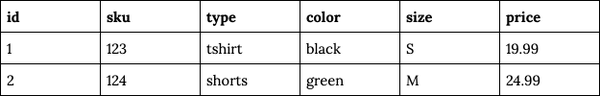
Figure 1-4. Row-wise storage, in which each row is stored together on disk

To reduce the width of tables, row-store databases are usually modeled in third normal form, which is a database design approach that seeks to store each piece of information only once, to avoid duplication and inconsistencies. This is efficient for transaction processing but often leads to a large number of tables in the database, each with only a few columns. To analyze such data, many joins may be required, and it can be difficult for nondevelopers to understand how all of the tables relate to each other and where a particular piece of data is stored. When doing analysis, the goal is usually denormalization, or getting all the data together in one place.

Tables typically have a primary key that enforces uniqueness—in other words, it prevents the database from creating more than one record for the same thing. Tables will often have an id column that is an auto-incrementing integer, where each new record gets the next integer after the last one inserted, or an alphanumeric value that is created by a primary key generator. There should also be a set of columns that together make the row unique; this combination of fields is called a composite key, or sometimes a business key. For example, in a table of people, the columns first_name, last_name, and birthdate together might make the row unique. Social_security_id would also be a unique identifier, in addition to the table’s person_id column.

Tables also optionally have indexes that make looking up specific records faster and make joins involving these columns faster. Indexes store the values in the field or fields indexed as single pieces of data along with a row pointer, and since the indexes are smaller than the whole table, they are faster to scan. Usually the primary key is indexed, but other fields or groups of fields can be indexed as well. When working with row-store databases, it’s useful to get to know which fields in the tables you use have indexes. Common joins can be sped up by adding indexes, so it’s worth investigating whether analysis queries take a long time to run. Indexes don’t come for free: they take up storage space, and they slow down loading, as new values need to be added with each insert. DBAs may not index everything that might be useful for analysis. Beyond reporting, analysis work may not be routine enough to bother with optimizing indexes either. Exploratory and complex queries often use complex join patterns, and we may throw out one approach when we figure out a new way to solve a problem.

Star schema modeling was developed in part to make row-store databases more friendly to analytic workloads. The foundations are laid out in the book The Data Warehouse Toolkit,² which advocates modeling the data as a series of fact and dimension tables. Fact tables represent events, such as retail store transactions. Dimensions hold descriptors such as customer name and product type. Since data doesn’t always fit neatly into fact and dimension categories, there’s an extension called the snowflake schema in which some dimensions have dimensions of their own.

Column-Store Databases

Column-store databases took off in the early part of the 21st century, though their theoretical history goes back as far as that of row-store databases. Column-store databases store the values of a column together, rather than storing the values of a row together. This design is optimized for queries that read many records but not necessarily all the columns. Popular column-store databases include Amazon Redshift, Snowflake, and Vertica.

Column-store databases are efficient at storing large volumes of data thanks to compression. Missing values and repeating values can be represented by very small marker values instead of the full value. For example, rather than storing “United Kingdom” thousands or millions of times, a column-store database will store a surrogate value that takes up very little storage space, along with a lookup that stores the full “United Kingdom” value. Column-store databases also compress data by taking advantage of repetitions of values in sorted data. For example, the database can store the fact that the marker value for “United Kingdom” is repeated 100 times, and this takes up even less space than storing that marker 100 times.

Column-store databases do not enforce primary keys and do not have indexes. Repeated values are not problematic, thanks to compression. As a result, schemas can be tailored for analysis queries, with all the data together in one place as opposed to being in multiple tables that need to be joined. Duplicate data can easily sneak in without primary keys, however, so understanding the source of the data and quality checking are important.

Updates and deletes are expensive in most column-store databases, since data for a single row is distributed rather than stored together. For very large tables, a write-only policy may exist, so we also need to know something about how the data is generated in order to figure out which records to use. The data can also be slower to read, as it needs to be uncompressed before calculations are applied.

Column-store databases are generally the gold standard for fast analysis work. They use standard SQL (with some vendor-specific variations), and in many ways working with them is no different from working with a row-store database in terms of the queries you write. The size of the data matters, as do the computing and storage resources that have been allocated to the database. I have seen aggregations run across millions and billions of records in seconds. This does wonders for productivity.

Tip

There are a few tricks to be aware of. Since certain types of compression rely on sorting, knowing the fields that the table is sorted on and using them to filter queries improves performance. Joining tables can be slow if both tables are large.

At the end of the day, some databases will be easier or faster to work with, but there is nothing inherent in the type of database that will prevent you from performing any of the analysis in this book. As with all things, using a tool that’s properly powerful for the volume of data and complexity of the task will allow you to focus on creating meaningful analysis.

Other Types of Data Infrastructure

Databases aren’t the only way data can be stored, and there is an increasing variety of options for storing data needed for analysis and powering applications. File storage systems, sometimes called data lakes, are probably the main alternative to database warehouses. NoSQL databases and search-based data stores are alternative data storage systems that offer low latency for application development and searching log files. Although not typically part of the analysis process, they are increasingly part of organizations’ data infrastructure, so I will introduce them briefly in this section as well. One interesting trend to point out is that although these newer types of infrastructure at first aimed to break away from the confines of SQL databases, many have ended up implementing some kind of SQL interface to query the data.

Hadoop, also known as HDFS (for “Hadoop distributed filesystem”), is an open source file storage system that takes advantage of the ever-falling cost of data storage and computing power, as well as distributed systems. Files are split into blocks, and Hadoop distributes them across a filesystem that is stored on nodes, or computers, in a cluster. The code to run operations is sent to the nodes, and they process the data in parallel. Hadoop’s big breakthrough was to allow huge amounts of data to be stored cheaply. Many large internet companies, with massive amounts of often unstructured data, found this to be an advantage over the cost and storage limitations of traditional databases. Hadoop’s early versions had two major downsides: specialized coding skills were needed to retrieve and process data since it was not SQL compatible, and execution time for the programs was often quite long. Hadoop has since matured, and various tools have been developed that allow SQL or SQL-like access to the data and speed up query times.

Other commercial and open source products have been introduced in the last few years to take advantage of cheap data storage and fast, often in-memory data processing, while offering SQL querying ability. Some of them even permit the analyst to write a single query that returns data from multiple underlying sources. This is exciting for anyone who works with large amounts of data, and it is validation that SQL is here to stay.

NoSQL is a technology that allows for data modeling that is not strictly relational. It allows for very low latency storage and retrieval, critical in many online applications. The class includes key-value pair storage and graph databases, which store in a node-edge format, and document stores. Examples of these data stores that you might hear about in your organization are Cassandra, Couchbase, DynamoDB, Memcached, Giraph, and Neo4j. Early on, NoSQL was marketed as making SQL obsolete, but the acronym has more recently been marketed as “not only SQL.” For analysis purposes, using data stored in a NoSQL key-value store for analysis typically requires moving it to a more traditional SQL data warehouse, since NoSQL is not optimized for querying many records at once. Graph databases have applications such as network analysis, and analysis work may be done directly in them with special query languages. The tool landscape is always evolving, however, and perhaps someday we’ll be able to analyze this data with SQL as well.

Search-based data stores include Elasticsearch and Splunk. Elasticsearch and Splunk are often used to analyze machine-generated data, such as logs. These and similar technologies have non-SQL query languages, but if you know SQL, you can often understand them. Recognizing how common SQL skills are, some data stores, such as Elasticsearch, have added SQL querying interfaces. These tools are useful and powerful for the use cases they were designed for, but they’re usually not well suited to the types of analysis tasks this book is covering. As I’ve explained to people over the years, they are great for finding needles in haystacks. They’re not as great at measuring the haystack itself.

Regardless of the type of database or other data storage technology, the trend is clear: even as data volumes grow and use cases become more complex, SQL is still the standard tool for accessing data. Its large existing user base, approachable learning curve, and power for analytical tasks mean that even technologies that try to move away from SQL come back around and accommodate it.

Conclusion

Data analysis is an exciting discipline with a range of applications for businesses and other organizations. SQL has many benefits for working with data, particularly any data stored in a database. Querying and analyzing data is part of the larger analysis workflow, and there are several types of data stores that a data scientist might expect to work with. Now that we’ve set the groundwork for analysis, SQL, and data stores, the rest of the book will cover using SQL for analysis in depth. Chapter 2 focuses on data preparation, starting with an introduction to data types and then moving on to profiling, cleaning, and shaping data. Chapters 3 through 7 present applications of data analysis, focusing on time series analysis, cohort analysis, text analysis, anomaly detection, and experiment analysis. Chapter 8 covers techniques for developing complex data sets for further analysis in other tools. Finally, Chapter 9 concludes with thoughts on how types of analysis can be combined for new insights and lists some additional resources to support your analytics journey.

¹ There are some newer technologies that allow SQL queries on data stored in nonrelational sources.

² Ralph Kimball and Margy Ross, The Data Warehouse Toolkit, 3rd ed. (Indianapolis: Wiley, 2013).