Deep Learning at Scale

Chapter 4. Putting It All Together: Efficient Deep Learning

In Chapter 2, you read about the fundamentals and data flows of deep learning applications. In Chapter 3, you learned about the various computational units that are available today and how they enable number crunching at scale. This chapter builds on the content from the previous two chapters, demonstrating the acceleration provided by specialized computing hardware and providing some examples of how-tos. It also presents some tips and tricks for efficiently training a deep learning model on a single machine with at most one accelerated device.

There are two hands-on exercises in this chapter, one using a language model (OpenAI’s GPT-2) and the second an image classification model (EfficientNet).¹ The GPT-2 exercise allows you to explore the level of acceleration a GPU provides and dig into the details of profiling tools to understand the underlying implications. In the second hands-on example, you’ll explore building a multiclass image segmentation solution using the MIT Scene Parsing Benchmark (SceneParse150) dataset. After you go through these exercises, you’ll look at several techniques you can apply to introduce efficiency in your code. More specifically, you will learn about graph compilation, mixed-precision training, efficiencies obtained via gradient tricks, memory layout tricks, and some DataLoader tricks to manage model input pipeline overheads. This chapter culminates with a small example of a custom kernel to demonstrate leveraging accelerated computing for custom operations.

Hands-On Exercise #1: GPT-2

ChaptGPT is an influential generative language model able to “converse” via free text prompts. The technology behind ChatGPT is OpenAI’s Generative Pre-trained Transformer (GPT), a large Transformer-based language model. Scale has been a crucial factor behind the success of GPT; it is a large model, trained with vast volumes of data, and it employs many tricks, some of which are known and will be discussed in Chapter 10. It was the second version of GPT, GPT-2, that achieved impressive success. In this exercise, you will explore that model.

The task for GPT-2 is to predict the next word given the previous words within some text. GPT-2 has more than 10x as many parameters and is trained with 10x more data than the original GPT. More concretely, GPT-2 has 1.5 billion parameters and is trained from the text extracted from 8 million web pages.

Note

GPT-2 was released in early 2019. Since then (as of early 2024) GPT-3, -3.5, and -4 have also been released, albeit kept closed source (with very limited sharing of implementation details). A comparison of the versions across different criteria is provided in Table 4-1, in “Key contributors to scale”.

Exercise Objectives

The objectives of this exercise are as follows:

• Review examples of how to write infrastructure-agnostic code. This allows you to easily scale out to other infrastructure in the event of a computing bottleneck.

• Profile and monitor to measure the behavior of your model and training loop. These skills are useful in understanding the limitations and provide clues to optimize appropriately.

• Learn about techniques to leverage hardware capabilities to develop efficiently.

• Optionally, learn about Docker and other build toolchains to build runtimes suited to your development needs, rather than using Swiss army knife environments like NVIDIA GPU Cloud (NGC) containers.

The following section explores the architecture of the model and the implementation details. (For a more thorough walkthrough, see Jay Alammar’s detailed explanation of GPT-2, which explains intricate concepts such as the Transformer, attention block, masked self- and cross-attention, and the role the query, key, and value play in predicting the possible next word/token).² The code for this exercise is available in the chapter_4 folder of the book’s GitHub repository.

Model Architecture

The key technique GPT employs is masking some words in the text corpus and training the model to predict the masked words by exploiting the remaining corpus of text. For example, the model might be shown the text “I brought a book to ___” and asked to predict the missing word, “read.” As you can see, there may be more than one word that could fit here (e.g., “learn”). These possible words need to be scored to identify the recommended word. With attention blocks, Transformer architectures can attend to longer sequences of tokens in a parallelized fashion. This, combined with this masking ability, allows the model to develop a better language understanding and exploit the semantic meaning of text via word embedding.

GPT-2 is a decoder-only autoregressive model. The full architecture is shown in Figure 4-1, including a breakdown of the GPT block (the decoder component). This figure demonstrates how the text embedding and positional encoding flow through the network, which consists of a series of multiheaded masked attention blocks, composed together with LayerNorm (layer normalization) and Conv1d (1D convolution) layers. You may note that this network has several residual connections throughout. The attention block has both self- and cross-attention, so (as shown in the bottom-right corner of the figure) either the query, key, and value can all come from the same text sequence, or the query can come from one sequence and the key and value from another.

Key contributors to scale

Let’s review some of the key features of GPT-2 that contributed to the scaling of this technique.

Transformer attention block

Ashish Vaswani et al. initially proposed the multiheaded attention block that is used in GPT in their seminal paper “Attention Is All You Need.”³ The key feature of this architecture is that the words of the text are processed as a whole. Other contemporary architectures, like recurrent neural networks (RNNs) and long short-term memory networks (LSTMs), process words one by one in a temporal sequence and remember the representation of these words through hidden states. The inability to process words in parallel was a key reason the capabilities of language models before Transformers were not rapidly improving. With the introduction of the Transformer, a larger context through a sequence of tokens/words could be provided. For GPT-2 this context size was 1,024 tokens, twice that of GPT (see Table 4-1). The context size has since been scaled up to a starting size of 8,192 tokens in GPT-4,⁴ and the reasoning abilities of this network have scaled proportionately.

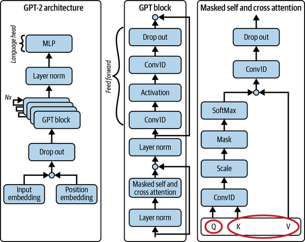
Figure 4-1. The architecture of GPT-2 and detailed breakdown of its subnetwork

Table 4-1. The evolution of various GPT models across versions

Name	Context size	Number of parameters	Layers	Depth of model	Comparable model (capacity-wise)
GPT-2 small	1,024	117M	12	768	GPT (original)
GPT-2 medium	1,024	345M	24	1,024	BERT
GPT-2 large	1,024	762M	36	1,280
GPT-2 XL	1,024	1,542M	48	1,600
GPT-3 small	2,048	125M	12	768	GPT-2 small
GPT-3 medium	2,048	350M	24	1,024	GPT-2 medium
GPT-3 large	2,048	760M	24	1,536	GPT-2 large
GPT-3 XL	2,048	1.3B	24	2,048	GPT-2 XL
GPT-3 2.7B	2,048	2.7B	32	2,560
GPT-3 6.7B	2,048	6.7B	32	4,096
GPT-3 13B	2,048	13B	40	5,140
GPT-3 175B	2,048	175B	96	12,288
GPT-4	8,192	Undisclosed (rumored to be 1.76T)	Undisclosed	Undisclosed
GPT-4-32k	32,768	Undisclosed	Undisclosed	Undisclosed

Unsupervised training

As discussed earlier, the training of GPT is achieved by masking certain tokens in the training dataset. Because of this technique, there is no labeling or supervision required for training these large language models. The training data thus remains easy to procure through a web crawler. Given the enormous amount of textual data available on the internet, it is only the quality of the inputs that remains a concern. OpenAI employs a filtering technique to choose pages of text that have received at least three user upvotes (“likes” of the page) more to ensure the quality of the content used to train the model. These scraped texts formed the vocabulary of GPT-2, which was also expanded to 50,257 from the 40,478 unique tokens used for training GPT.

Zero-shot learning

In the initial version of GPT, OpenAI focused on training a large language model through pretraining and fine tuning different versions of the model for various language purposes like question answering, text summarization, language translation, and reading comprehension. However, because the semantic relations between words remain consistent across applications of spoken language, with GPT-2 it was noted that the model could be repurposed for such tasks via zero- or few-shot techniques (discussed in Chapters 11, 12, and 13). In other words, it’s possible to train a very good language model and repurpose it for various tasks at inference time. This is achievable because zero-shot techniques do not require backpropagation; thus, repurposing is highly cost-, compute-, and time-efficient.

This is a very important aspect of GPT that should be considered seriously for model development across related tasks. Repurposing an existing model for a related task via fine tuning or inference-time alignment, as in meta-learning and zero-shot learning, is a great optimization trick. This will be covered in detail in Chapter 11.

Parameter scale

As discussed already, GPT-2 is simply a scaled-up version of GPT (with a slight rearrangement of the LayerNorm layers). The scale in GPT-2 comes from the use of a larger context size and more GPT blocks (Figure 4-1 and Table 4-1). The subsequent versions of the model continued to scale; the largest GPT-3 model, for example, has 175 billion parameters.⁵ For reference, humans are estimated to have 100 trillion synapses.

Implementation

Although the code for GPT-2 has been open sourced by OpenAI, in this exercise, you will be using Hugging Face’s Transformers library, which provides a PyTorch implementation of the GPT-2 architecture shown in Figure 4-1. Specifically, you will be using the library’s GPT2LMHeadModel, a GPT2 model transformer with a language modeling head on top.

For wiring up GPT-2 you will use PyTorch Lightning, as in Chapter 2. You’ll use the Hugging Face wikitext dataset for training.

As mentioned earlier, the code for this hands-on exercise is available in the book’s GitHub repository. The implementation is explained in the following sections.

model.py

The model implementation in this script is straightforward, as most of the complexity of the model is abstracted away in GPT2LMHeadModel. The model input pipeline tokenizes the text, and the forward call is dispatched to the GPT2LMHeadModel, which returns the cross-entropy loss between the predicted token and the true token. This script wraps the model from the Transformers library in the Lightning abstraction of LightningModule.

dataset.py

The dataset implementation is in WikiDataModule, which wraps v2 of the wikitext dataset. In this module, the raw text is downloaded, preprocessed, tokenized, and then grouped according to the block capacity of the model. The data is split into training, validation, and test sets and a respective DataLoader is created for each of the modules.

app.py

The trainer code is included in app.py. Note specifically the entry point method train_gpt2, which defines various components integrated into the training regime, including callbacks and profilers (much like the hands-on PyTorch exercise in Chapter 2). The profilers should only be used during development and formal runs as they incur costs in terms of memory and compute resources. The trainer code is as follows:

datamodule = WikiDataModule(name=model_name, batch_size=batch_size, 
                            num_workers=num_workers)
model = GPT2Module(name=model_name)

trainer = PLTrainer(
    accelerator="auto",
    devices=="auto",
    max_epochs=max_epochs,
    callbacks=[
        TQDMProgressBar(refresh_rate=refresh_rate),
        ckpt_cb,
        DeviceStatsMonitor(cpu_stats=True),
        EarlyStopping(monitor="val/loss", mode="min"),
    ],
    logger=[
        exp_logger,
        TensorBoardLogger(save_dir=result_dir / "logs"),
    ],
    profiler=torch_profiler,
)
trainer.fit(model, datamodule)

Notice the accelerator and devices arguments in this code. These parameters provide the ability to write platform-agnostic code so the same code can be run on CPUs, GPUs, TPUs, or other assorted accelerators. It also supports computation on Metal shaders, available in Apple’s M-series GPUs. In other words, this snippet allows you to tick off the first objective of writing platform-agnostic code that you can run anywhere and scale out per your needs.

Note

There are a few other ways to do this, including using Hugging Face’s Trainer, which provides a similar capability. However, for the sake of consistency and reusability, in these exercises PyTorch Lightning will be used as an orchestrator.

Running the Example

To run the code, execute the following command from your environment:

deep-learning-at-scale chapter_4 train_gpt2

Following are some examples of the results obtained after training this model on the wikitext dataset for 50 epochs. The prompt used was “I’ve been waiting for a deep learning at scale book my whole life. Now that I have one, I shall read it. And I.” Here’s some of the generated text:

• I have a feeling that it’s going to be a long time before I retire from this.

• ive learned so much from it.

• ive no doubt that it’s going to change my life.

• I’ll be ready to do anything I can to help it. I’ll be on the…

• ’ ll be able to do anything I would normally do in life.

• ive to see how it all plays out.

• ive been waiting for a deep learning book for a long time.

• will be able to see what I can do to make it happen.

Experiment Tracking

This practice exercise (and others throughout this book) uses Aim, an open source experiment tracking solution, to monitor and visualize the progress and metrics of training runs. I chose Aim as it’s free to use with no commitment from you. There are, however, several alternatives that you can use instead, as you see fit. Some of these alternatives will be briefly discussed in Chapter 11 (see “Setting Up for Iterative Execution”). The following snippet is used to enable the experiment tracking logger:

exp_logger = AimLogger(
    experiment=exp_name,
    train_metric_prefix="train/",
    val_metric_prefix="val/",
    test_metric_prefix="test/",
)

This logger is then configured with the trainer API as logger: i.e., trainer = Trainer(... , logger=[exp_logger]), as shown in the earlier Trainer snippet.

Note

You will have to start aim server locally by running command aim up to visualize the run logs in aumhub. Your runs will log both profiler logs and run logs that you can visualize using tensorboard and aimhub respectively (as done in Chapter 2). Results shown in Figures 4-2 and 4-3 can be visualized using these two tools.

Measuring to Understand the Limitations and Scale Out

This section presents the performance measures obtained by running the code on a high-end CPU and a GPU and compares the two to explore the limitations.

Running on a CPU

Figure 4-2 shows the results obtained when this code was run on a nonaccelerated computer with a 10-core CPU and 32 GB of memory (RAM). The batch size used in this run was set at 12.

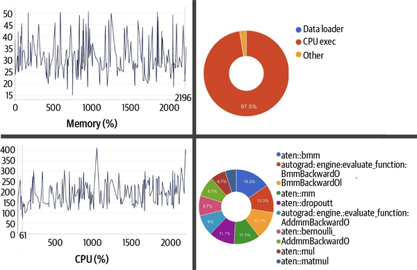
Figure 4-2. Screen grabs of resource usage and operator profiling obtained from the run of this example when trained on CPU-only compute

The average time to take one step (i.e., process one batch of data and do forward and backward passes) was about 304 seconds, with 97.46% of this time spent executing operations on the CPU and 2.54% spent on non-CPU operations. Noticeably, negligible time was spent to support the data loading operations (e.g., loading the wikitext dataset in memory for execution).

The profiler’s memory consumption graph indicates a peak at 42.64 GB; however, if you look at the continuous monitoring of memory usage, in Aim’s system metrics in this case, you may note the peak sits at 50 GB.

Tip

Profilers are configured to sample steps during which the profiling should be run. You can see this in the schedule configured for the profiler in this example, torch.profiler.schedule(wait = 1, warmup = 1, active =5, repeat = 10, skip_first = True). This is useful to minimize the overhead of profiling on the run, but it poses the risk of not capturing the usage appropriately. This is why high-level continuous monitoring is useful and schedule settings should be tweaked to ensure you get good coverage.

The system metrics also indicate that CPU utilization peaked at 410% in this run. Observing the main process via a tool like htop shows that it has a virtual size of a whopping 453 GB, which includes the physical memory, swap memory, files on disk that have been mapped into the process (e.g., shared libraries), and shared memory space (shared with other processes, for example).

Figure 4-2 shows the top 10 operations that took the longest time to compute, with the batch matrix-to-matrix operation aten::bmm accounting for the largest percentage of the time, at 15.2%. Increasing the batch size would allow you to reduce the total number of steps (that is, the total number of times this operation needs to be called per epoch).

At a batch size of 12, the total number of steps sums to 184. Hypothetically speaking, if the batch size were to be doubled to 24, the number of steps would be reduced to 92. Given the vectorized nature of the aten::bmm operation, if you had more compute cycles available, doubling the batch size would effectively halve the cost of this computation. However, as you increase the batch size the memory requirements to hold the input tensor (the token embedding) will increase, and so will the amount of memory required to hold the gradients. The gradients’ memory requirement scales linearly with batch size; that is, the space complexity is given by O(batch_size). The implication for sample-wise losses and metrics would also increase in the same order.

For this reason, it’s important to find the optimum balance between CPU and memory (both physical and virtual). In this instance, on the available CPU hardware, using a batch size of 24 was simply not possible as the system was running into out-of-memory (OOM) issues. In fact, even with a batch size of 12 the host system was sporadically unresponsive. There are autotuning techniques like Torch Memory-adaptive Algorithms (TOMA) that can find the most suitable batch size by retrying with a lower size if OOM errors occur; using these tricks can remove the manual overhead of right-sizing the batch size, and they can be easily enabled by using the light⁠ning.pytorch.tuner.Tuner.scale_​batch_size() API.

As discussed in Chapter 3, managing the memory requirements by reducing the precision of the tensors is also an option; however, standard CPUs do not have specialized hardware for the various floating-point formats mentioned there. Accelerator units are more specialized in data crunching and have additional hardware to support lower-precision compute; CPUs are general-purpose hardware where this support is largely absent or emulated.

Given that at a batch size of 12 the system was sporadically unresponsive and took an average of 304 seconds to complete one step, it would take about 15.5 hours to finish one epoch (184 steps). Function tracing, as provided by a profiling tool such as the PyTorch profiler used in this example, is very helpful in understanding the duration and nature of operations that are occupying the process space (see Figure 4-3). This is useful in identifying suboptimal calls for further optimizations.

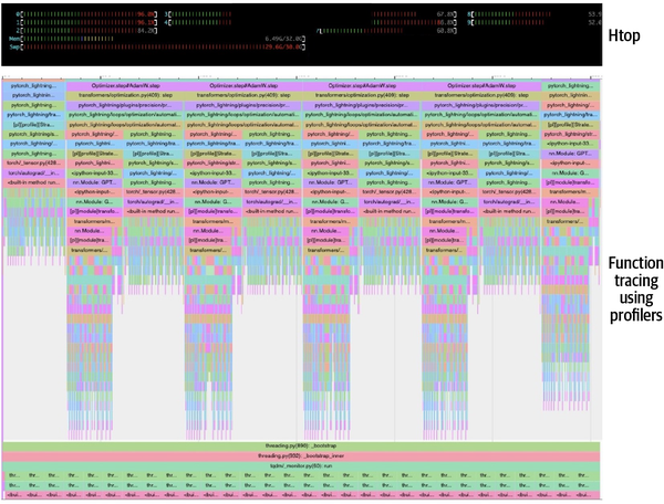
Figure 4-3. Function tracing provided by the PyTorch profiler when this example is run on a CPU

The main takeaway from this exercise is that right-sizing the memory and number of CPU cores and tuning the batch size will help you to get the best out of CPU-based training. However, the turnaround time for deep learning on a CPU may be insufficient—15+ hours for one epoch, as in this case, is a very impractical feedback cycle for rapid development and a good user experience.

In this following section, we’ll look at how this example can be scaled out on a heterogeneous computer using a CPU similar to the one used in this section in conjunction with an NVIDIA A100 80 GB GPU.

Running on a GPU

In Chapter 3, you read about the execution model for accelerated computing and learned how the host/CPU facilitates operator (i.e., kernel) execution on a GPU in a parallelized fashion. You also learned about the steps involved to transfer data from the host into GPU memory and the overhead this may cause because of limited bandwidth.

In this exercise, the model input (data) pipeline loads the text data in memory, performs preprocessing and tokenization, and generates the embedding, as shown in Figure 4-1. These embeddings—the matrix tensors—are loaded into the GPU’s VRAM. Then, as the computation proceeds, various kernel functions are called on the GPU to perform the required operations in a vectorized fashion over its thousands of cores.

Figure 4-4 is a screen grab obtained from a function trace of a training run of this example on an NVIDIA A100 SXM 80 GB GPU. The top trace pertains to a thread, spun up by the main process, that handles communication between the device and the host. This trace also shows another thread on the same host that manages the CPU-bound computations (e.g., the model input pipeline). The bottom part of the figure shows the stack for the thread corresponding to GPU computation. Note the corresponding dip in the streaming multiprocessor when the memory copy operations are in flight. The lowest row indicates the elapsed time for each of the kernel functions invoked during the stages of profiling. Notice how different the tracing obtained from a CPU and a GPU is (Figures 4-3 and 4-4, respectively).

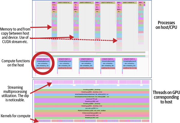
Figure 4-4. Function tracing provided by PyTorch profiler when run on a GPU

To run this example on a GPU, you can use the same command you used to run it on a CPU (see “Running the Example”). Because the code is written to be platform-agnostic, no changes are needed. However, you will need to ensure that your hardware has an NVIDIA driver and runtime installed. Since one of the goals of this exercise is to be able to monitor the usage, you’ll also need to have the CUDA Profiling Tools Interface (CUPTI) installed. For pointers to the complete setup instructions, refer to “Setting Up Your Environment for Hands-on Exercises”.

Note

CUDA kernel profiling tools like CUPTI and NVProf are extremely helpful, but they only provide operator/kernel-level profiles. Unfortunately, they do not provide a higher-level perspective such as of the neural layer. This contextualization needs to be done by the user.

The first observation to make when running this exercise on an A100 80 GB GPU is that the memory utilization of the host has dropped significantly to marginal. In addition, at a batch size of 12 only about 40 GB of VRAM on the GPU is used. Also noteworthy is that the average step time has dropped to 4 s from 304 s on a pure CPU run. As you can see in Figure 4-5, GPU utilization is at 94.5%, with 0.4% used for memory copy, 1.5% for CPU-bound operations, and 3.7% for other operations. Notably, DataLoaders continue to account for a marginal fraction of this.

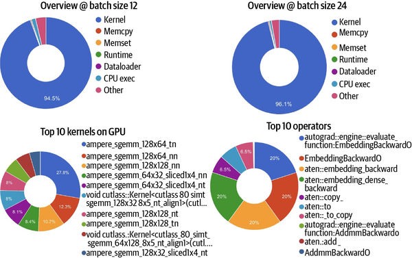
Figure 4-5. Screenshots of function/operator tracing and GPU kernel profiling obtained from the run of this example when trained on heterogeneous compute with an NVIDIA GPU

We have 80 GB and only 50% is used. Let’s now increase the batch size to 24. The ideal utilization should be 100%, in theory, indicating all cores are being utilized at max capacity. At a batch size of 24, there is an increase of less than 2% in GPU utilization (to 96.1%), as shown on the right in Figure 4-5. There is a corresponding drop in CPU execution and “other” operation.

Looking at the bottom of Figure 4-5, we can see that when a GPU is brought into the mix the longest-running operator is no longer aten::bmm (as in the case of the CPU-only run, shown in Figure 4-2). Now, the most expensive operation is autograd::engine::evaluate_function:EmbeddingBackward0, which pertains to gradient computation during automatic differentiation (i.e., backward propagation). The reason for this difference is that the batch matrix-to-matrix operation aten::bmm is much more easily scaled out on a GPU, and the turnaround drops massively because of parallelization. This is essentially a good application of Amdahl’s law, since the scalable part of the computation—the matrix operation—is parallelized. Other expensive operations are related to copying, which is indicative of the challenges with memory loads.

As expected, as batch size increases, an increase in GPU utilization and a decrease in step time are observed. However, there is no impact on the order of top operations. The trace, as shown in Figure 4-5, continues to be similar, albeit with an increase in the utilization stats.

As discussed in Chapter 3, most modern accelerators, including NVIDIA GPUs, come with computation units for various precision formats. The A100 specifically comes with Tensor Core units capable of estimating the appropriate level of precision and executing at that level. The three available modes, highest, high, and medium, pertain to decreasing orders of internal precision, with the highest level ensuring the use of single-precision floating-point numbers (32-bit). Using the following configuration to activate this capability, you will notice a time savings of about 0.7 s per step at the medium precision level, for a new average step time of 3.3 s:

torch.backends.cuda.matmul.allow_tf32 = True
torch.set_float32_matmul_precision("medium")

As the profiler indicates, only about 37.6% of the GPU computation used the Tensor Core, indicating other operators were perhaps not compatible with the tf32 format. This level of understanding is really helpful in optimizing the training run because it clarifies where most of the compute and memory expense is and, if critical, allows alternatives to these to be explored.

If you compare the model’s accuracy with and without tf32 enablement, you’ll find that the impact of the loss of precision is negligible in this case. However, depending on your circumstances, it can be worth making this trade-off. This trick uses the Tensor Core architecture, which is specific to NVIDIA’s Ampere and later GPU series. If your hardware is not equipped with Tensor Core capability, simplifying using standard-precision formats like fp16 or mixed fp16 may provide a significant gain too. We’ll talk more about this in “Mixed precision”.

Tip

The activation of tf32 compute overlaps with mixed-precision training. Depending on the tf32 support of the operators used in your model, the use of mixed precision in addition to enabling tf32 may provide advantages, but how much is dependent on your model and its functions.

Transitioning from Language to Vision

The exercise discussed here covers many aspects of language models. Before the Transformer architectures, the nuances of input modality (e.g., text, vision) drove the core modeling techniques and required specialized knowledge in dealing with domains specific to different input types. Just as sequence models dominated the language domain, convolution techniques were heavily used in computer vision models. The use of different modeling techniques per input modality is now reducing, as Transformers are emerging as a ubiquitous technique with applicability across input modalities. Transformer-based architectures like Vision Transformer (ViT)⁶ and Masked-attention Mask Transformer (Mask2Former)⁷ are proving performant. Transformer networks have quadratic computation complexity with regard to the input dimension, however, which when applied to multimedia contents such as pixelated images explodes the resource requirements. Depending on the complexity of the task at hand, convolutional architectures may provide computationally less demanding yet efficient implementations.

The following section focuses on a computer vision exercise, using the convolution technique.

Hands-On Exercise #2: Vision Model with Convolution

The task for this exercise is to generate segmentation results for the images in the MIT Scene Parsing Benchmark (SceneParse150) dataset, which are annotated with 150 categories of objects. Accounting for background or unknown, in total, you will be segmenting for 151 classes. This exercise demonstrates the scale channel where the number of classes for which you are segmenting is fairly large.

Model Architecture

This exercise leverages convolutional neural networks (CNNs), a computer vision–based deep learning technique. More specifically, you will be using EfficientNet as a feature encoder and Convolve as a decoder blocker, assembled into a U-Net-based architecture.⁸

Key contributors to scale in the scene parsing exercise

Let’s take a closer look at some of the key techniques used in this exercise. These techniques help with scaling to process large images for large numbers of classes in an efficient and scalable manner.

Scaling with convolutions

One of the main challenges when working with images is the scale of input. A 512x512 three-channel (color) image will have an input vector of size 786,432. The size of the input vector increases linearly with the increase in height or width of the images. However, these inputs are not independent; there is also a structural (spatial) and textural correlation that exists in the images. With a motivation to develop more efficient techniques to learn from images, convolutional networks were envisaged to exploit this correlation of image feature properties, leveraging sparsity and parameter sharing.

CNNs, first proposed by Yann LeCun in the 1980s,⁹ were inspired by the computer vision technique “convolving,” heavily used in image processing techniques like edge detection, blurring, etc. These techniques apply predetermined filters F of size fxf over the image in a sliding window operation shifting by stride s, effectively reducing the number of operations by a factor of s. This filtering operation is translation invariant because the same filter—say, the edge detection filter F—can be used to extract an edge from anywhere in the image (in the center, along an edge, or otherwise). The filters of the convolution layers (as in deep learning) are learned during backpropagation. The reusability of these learned filters F (see Equation 4-1) makes CNNs quite interesting and highly optimized, as not only is the number of parameters required in a CNN massively reduced, but they’re also shared across each stride. This phenomenon is commonly known as weight sharing. Andrew Ng’s Stanford CS230 lecture notes and Piotr Skalski’s “Gentle Dive into Math Behind Convolutional Neural Networks” are good sources to explore the working of convolution layers further.¹⁰

Equation 4-1. Mathematical formula used by convolution layers for feature extraction from images

${\sum }_a^{f-1}{\sum }_b^{f-1}{F}_{ab}{x}_{(i+a)(j+b)}$

The architecture of LeCun’s CNN, LeNet-5, is shown in Figure 4-6.

Figure 4-6. LeNet-5 architecture (Source: https://alexlenail.me/NN-SVG/LeNet.html)

Scaling with EfficientNet

EfficientNet, as the name indicates, is a neural network architecture that uses compound scaling, as shown in Figure 4-7, to scale out convolutional models in an efficient manner. It combines scaling across depth, width, and resolution in a more effective way to obtain a more performant model that maximizes resource use. EfficientNet was developed using a technique called neural architecture search (a subfield of AutoML) that you will read about in Chapter 11.

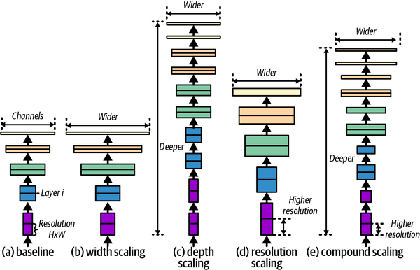
Figure 4-7. EfficientNet architecture (adapted from Tan and Le, 2019)

Implementation

As mentioned earlier, the final architecture used in the exercise is U-Net,¹¹ which uses EfficientNet as a backbone (see Figure 4-8).

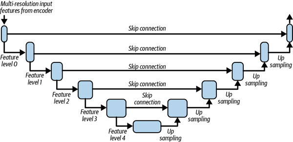
Figure 4-8. U-Net architecture (adapted from Ronneberger et al., 2015)

The code for this exercise is located in the chapter_4 folder of the book’s code repository. Let’s take a look at the implementation:

vision_model.py

The model implementation is in UNetSegmentationModel. It wires up the EfficientNet encoder from the Hugging Face library timm and connects it with another head designed for the segmentation task. This head, the Decoder, acts as a feature decoder tasked with generating segmentation output. The EfficientNet encoder provides multilevel features that are combined with the decoder outputs in a hierarchical fashion, as shown in the U-Net skip connection architecture (see Figure 4-8).

As in the previous exercise, this example uses PyTorch Lightning to leverage its ability to write infrastructure-agnostic code. The VisionSegmentationModule provides the LightningModule implementation.

dataset.py

The dataset implementation is in the SceneParsingModule, which wraps the SceneParse150 dataset. Note the specialized transformation used in this case to handle converting the images to tensors.

app.py

The entry point to this exercise is defined in app.py, in the method train_vision_model. Notice the use of VisionSegmentationModule and SceneParsingModule here. Otherwise, the implementation for this entry point is very similar to the previous exercise’s entry point, train_gpt2.

Running the Example

To run the code for this example, execute the following command from your environment:

deep-learning-at-scale chapter_4 train_efficient_unet

Observations

The maximum number of samples that can fit in the memory of an A100 80 GB GPU is 85. On the baseline run of this sample, an average step time of 3.3 s per iteration can be achieved. This is higher than the step time observed in the GPT-2 example. One reason for the high latency is that a very large volume of data (85 images) is read, decoded, and further processed, creating an I/O-intensive process. This is a common challenge for vision-based modeling tasks.

We’ve now gone through two hands-on examples and explored various techniques they employ to develop efficient and effective models. In the following sections, you will learn about some orthogonal techniques to speed up your training code and explore the trade-offs of these techniques.

Graph Compilation Using PyTorch 2.0

As discussed in Chapter 2, PyTorch is a dynamic graph computation engine that incurs an additional cost of graph compilation. As you saw in Chapter 3, this cost is usually relatively small compared to the cost of the matrix computation required by the network—but as accelerators are getting faster, this gap is narrowing. Also, as deep learning practices are evolving, more practitioners are writing custom accelerated/GPU kernels to speed up their code. Ease of use is the first principle in the design of the PyTorch framework and APIs. However, the C++ development required for CUDA kernels reduced their usability for the deep learning practitioners who needed custom CUDA operators.

PyTorch 2.0 addresses both of the aforementioned challenges through its innovative approach to providing better performance and supporting dynamic tensor shapes while being backward compatible. These capabilities are realized by making compiler-level changes for graph execution. The frame evaluation API added to CPython in Python 3.6 via PEP 532 (also discussed in Chapter 2) has been critical in this design.

New Components of PyTorch 2.0

To provide this graph-compilation capability, four new components were added in PyTorch 2.0: PrimTorch, TorchDynamo, AOTAutograd, and TorchInductor. PrimTorch is a simplified minimal set of primitive operators that facilitates writing complex operators in Python. The main emphasis of this component is to support easier development of custom hardware-specific kernel functions that would otherwise have required complex C++ development with a corresponding CPython interface for Python.

TorchDynamo is an effort to provide graph compilation capability without losing usability by tracing dynamically using Python bytecode transformation. TorchScript, as mentioned in Chapter 2, followed a similar philosophy of tracing the graph to obtain a more efficient variant. However, TorchScript is limited in its ability to handle control flows. PyTorch offers a few other tracing utilities, like torch.fx and PyTorch/XLA, but the key difference with TorchDynamo is the use of the frame evaluation API. In fact, torch.fx has now been migrated into TorchDynamo (see Figure 4-9).

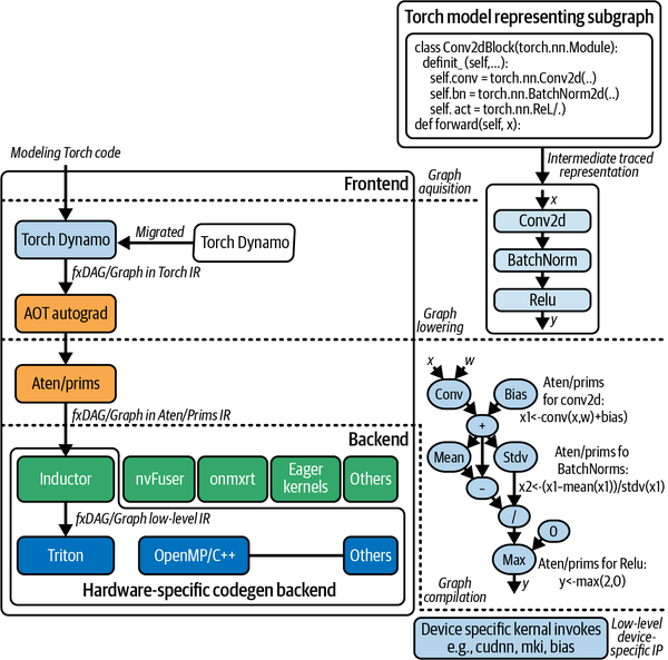
Figure 4-9. Key components of PyTorch 2.0 facilitating the ability to produce compiled graphs

Graph Execution in PyTorch 2.0

Graph execution in PyTorch 2.0 consists of three steps: graph acquisition, lowering, and compilation. Let’s take a look at each of these in turn.

Graph acquisition

Your model computation graph is composed using a set of subgraph (i.e., torch.nn.Module) implementations. These subgraphs are compiled and consolidated (flattened) by one of the many backends of TorchDynamo (aot_ts_nvfuser, cudagraphs, inductor, ipex, nvprims_nvfuser, onnxrt, tvm), where possible. This compilation saves the overhead of generating graphs dynamically on every iteration (as is done in PyTorch 1.x, as discussed in Chapter 2). The caveat here is that, because of the Pythonic nature of PyTorch, not all of your control flow operations can be compiled into graphs or subgraphs. These unsupported parts of your control flow are integrated into the execution phase by falling back to eager mode. This seamless switching, made possible by the frame evaluation API, offers an effective technique to leverage the graph compilation capability of PyTorch 2.0. The efficiency it provides without losing ease of use while still being Pythonic is great. The PyTorch Dev Discussion thread “TorchDynamo: An Experiment in Dynamic Python Bytecode Transformation” discusses the internals in greater detail.

The following snippet demonstrates how the trace is realized using conv_block, which we used in the earlier vision exercises:

from torch.fx import symbolic_trace
symbolic_traced : torch.fx.GraphModule = symbolic_trace(conv_block)

The internal representation obtained via PyTorch’s trace is shown here. This is another representation of the graph computation shown in Figure 4-9:

print(symbolic_traced.graph)
graph():
    %x : [#users=1] = placeholder[target=x]
    %conv : [#users=1] = call_module[target=conv](args = (%x,), kwargs = {})
    %bn : [#users=1] = call_module[target=bn](args = (%conv,), kwargs = {})
    %act : [#users=1] = call_module[target=act](args = (%bn,), kwargs = {})
    return act

The same graph, visualized in tabular format, is shown here, indicating the connectivity between the operations and input and outputs:

symbolic_traced.graph.print_tabular()
opcode       name    target    args     kwargs
-----------  ------  --------  -------  --------
placeholder  x       x         ()       {}
call_module  conv    conv      (x,)     {}
call_module  bn      bn        (conv,)  {}
call_module  act     act       (bn,)    {}
output       output  output    (act,)   {}

Graph lowering

In the graph lowering stage, all the graph operations are decomposed into their constituent kernels, specific to the chosen backend. In this step, the internal representation (IR) of the graph is obtained. PyTorch’s ATen and primitive components, a.k.a. prims, handle this stage. At this stage, the graph is more aligned/prepared for hardware-specific invocation.

Graph compilation

The graph compilation phase is when the kernels from the IR obtained in the preceding phase get translated to their corresponding low-level device-specific operations. This phase requires the backend to perform the compilation and also execute device-specific kernels. TorchInductor (a.k.a. inductor), the default engine for compilation, uses OpenAI Triton under the hood. However, other backends (such as aot_ts_nvfuser, cudagraphs, ipex, nvprims_nvfuser, onnxrt, and tvm) are also being actively developed.

In Chapter 2, you learned about the data flow of deep learning and compute requirements for arithmetic operations. In this section, you looked at clever improvements in PyTorch to mitigate dynamic graph inefficiencies. In the following section, we’ll explore tricks and techniques, including graph compilation, that can be employed to train models efficiently on a single device.

Modeling Techniques to Scale Training on a Single Device

Most of the techniques described in this section are orthogonal and can be applied in combination or independently. These techniques can help you achieve efficiency by increasing computational speed or reducing memory requirements.

Graph Compilation

To leverage the advantages of using a compiled graph, use the orthogonal API torch.compile. Applying torch.compile on torch.nn.Module converts it to the OptimizedModule type, an internal representation for optimized graph modules. As per the benchmarks documented in PyTorch issue #93794, this provides a 30% to 200% gain in performance depending on the type of architecture and underlying implementation.

The argument fullgraph is used to generate a static graph without eager mode fallback between the subgraphs. If your module does not have control flow (if/else and other conditional flows), then your chances of obtaining this type of graph will be higher. In general, using fullgraph will be a more efficient approach wherever possible. You can also choose your backend, as discussed previously; this defaults to inductor (see Figure 4-9).

There are three modes of compilation:

default

The default mode compiles the graph using the chosen backend, but does so efficiently without taking too much time or memory. In general, this mode will be more advantageous for large models.

reduce-overhead

This mode aims to remove overhead from the underlying framework and thus takes longer to compile and uses a small amount of extra memory. The reduce-overhead mode is more effective if your model and step inputs are smaller.

max-autotune

As the name indicates, this mode aims to provide a compiled graph with maximal tuning, which is thus faster. However, the compilation phase will be the longest of the three.

To see the difference before and after compilation, set the mode parameter, as shown here:

torch.compile(self.model, mode = "max-autotune")

and execute the following command from your environment:

deep-learning-at-scale chapter_4 train_gpt2 ––use-compile

To observe the standard eager mode behavior, which is also the default behavior of the example script, run the same command with -–no-use-compile instead.

Tip

If you run into issues with compilation or notice suboptimal performance, using the environment variable TORCH_LOGS=​"graph_breaks,recompiles" may help with debugging.

When running this example on an A100 SXM 80 GB GPU, you may note that at single precision (fp32), 24 is the optimal batch size for training. A batch size bigger than 24 will lead to OOM errors. You’ll also find that by compiling the graph with the default option, you can get a 5% gain in the efficiency of your training compared to the baseline non-compile eager mode computation. Changing the mode to max-autotune will bump the gain to 12%. As the TorchDynamo error logs may indicate, the network is not fully Dynamo-compliant (due, for example, to the use of list objects). Fixing these errors will provide a higher gain in efficiency. Generally, the use of lists in training should be discouraged, especially in DataLoaders, as they can cause memory blowout due to how Python multiprocessing pickles list objects (see PyTorch issue #13246 for a discussion of this issue).

One of the techniques you can use to move from lists to tensors is to stack them (i.e., using torch.stack([...])), if they are of the same dimensions. Otherwise, you can add padding to obtain a max-size stacked tensor. If your use case is specialized and neither of those tricks helps, you can try writing custom objects with suitable handling to implement the .to() method to handle device transfer.

In this section, you learned about a one-liner trick to gain about a 15% increase in efficiency. In the following section, you will explore how to gain more speed at the expense of precision.

Reduced- and Mixed-Precision Training

The memory consumed during training can be classified into two categories: memory consumed by model states and by residual states. We’ll talk more about this in Chapter 9, but for now let’s focus on the memory requirements during training in absolute form. These are determined by the following categories of numeric data, which are loaded in memory:

• Model parameters (weights and biases)

• Input data (generally loaded in chunks in memory)

• Activations/feature map (the results of the computations; i.e., the features extracted from the input data)

• Gradients (the error gradients required for backpropagation and error correction)

• Optimizer states (estimated to occupy 33–75% of memory)¹²

• Metrics and losses (numeric values to observe and monitor the progress of the training regime)

While the activation memory requirements are transitional, they scale linearly with the number of model parameters and size of the input data. Likewise, the memory requirements for backpropagation (i.e., gradients) increase linearly with batch size and number of parameters. Metrics and losses, in general, have negligible memory requirements. However, depending on the nature of the metrics (e.g., micro or macro), the requirements can scale on the order of the model’s task objective. For example, storing metrics for a simple binary classifier will require much less space than storing micro-metrics for the 151-class multiclass/multilabel classifier we looked at earlier in this chapter. Likewise, for object detection/localization tasks such as semantic or instance segmentation, the metrics requirements might be extensive (e.g., MaskIoU and mean/average/precision calculation for various object sizes, as is done in Mask R-CNN models).

Training is typically done using the standard single-precision floating-point format (fp32). Various less precise formats, as listed in Table 3-1 in “Floating-point standards”, can be used to speed up training, both by increasing the batch size (by reducing memory requirements as a result of the required data containers) and by leveraging the capabilities of hardware-optimized computation devices. Using a lower-precision format (e.g., fp16) may lead to suboptimal models. However, in scenarios where a highly precise outcome is not critical, the gain in efficiency achieved by reducing precision can be huge.

Mixed precision

Mixed precision, a technique that combines single- and half-precision floating-point formats, can also be used to manage the trade-off between computational efficiency and numerical accuracy. The Torch package torch.cuda.amp provides an implementation that enables the use of mixed precision for CUDA-compatible devices. Automatic mixed precision is realized by the torch.cuda.amp.autocast feature, which can manage data type conversions automatically. The Tensor Core architecture used in NVIDIA’s Ampere and later GPU series can also multiply half-precision matrices, accumulating the result in either a single- or a half-precision output. All of these techniques facilitate mixed-precision training.

Tip

When using automatic mixed precision, you should refrain from explicitly casting your tensors to any specific data type. Explicit casting hinders the automatic precision conversion, leading to suboptimal results.

There is a small memory penalty associated with mixed-precision training, because two copies of the model weights are loaded: one at single precision and the other at half precision. In effect, the memory requirements amount to 1.5x the requirements at single precision. Mixed precision is already implemented in the torch.cuda.amp and Lightning libraries, so you can enable it merely by calling Trainer(precision = "16-mixed").

Note

Mixed precision is primarily an accelerated device feature. The standard CPU computers do not offer lower-precision compute capabilities. As a result, you will note that automatic mixed precision is generally supported only for training on heterogeneous systems. Mixed precision is also a relatively new implementation (introduced around 2017); as a result, older GPUs may not have support built in for such training.

The effect of precision on gradients

Because gradients are calculated based on the error factor (i.e., the contribution of the parameters to the error), the value can be either too small or too large. Too large a gradient results in overflowing values, leading to numerical instability in computation. This phenomenon is termed the exploding gradients problem.¹³ As the numerical precision decreases, the capacity to hold a larger mantissa reduces, resulting in a higher risk of numerical overflow. Likewise, the capacity to hold very precise floating-point differences decreases, leading to an increased risk of underflow. Neither of the two scenarios is nice to have. Gradient scaling and clipping are two techniques that help avoid overflow and underflow issues during backward propagation.

Gradient scaling

PyTorch’s gradient scaler, as the name indicates, scales out gradients to manage the precision loss. Generally, the scaler is initialized:

scaler = torch.cuda.amp.GradScaler()

and used during the training loop to scale the loss before backpropagation:

scaler.scale(loss).backward()

Frameworks like Lightning automatically take care of gradient scaling when mixed precision is used. This is why you may note that this chapter’s hands-on examples do not feature an explicit use of GradScaler.

Gradient clipping

Gradient clipping is used to mitigate exploding gradients. Typically, the clipping is performed either on the value of the gradient or the norm of the gradient. In effect, it caps the maximum value (or norm) of the gradient during the training loop.

Lightning comes with a clip_gradients capability that can be activated via the infrastructure wiring code (e.g., by using Trainer(gradient_clip_val = 0.5)) and can be further customized using the configure_gradient_clipping function override of your LightningModule. You can find more detailed information in the documentation.

8-bit optimizers and quantization

As discussed previously, the data containers for gradients, even in mixed-precision training, are kept at fp32. Efforts to change the gradient precision to fp16 have proven to lead to less than desirable results, because the variance in gradients can be large (depending on how each of the parameters contributes to the error). The challenge with gradient scaling and clipping is that both of these tricks are applied consistently across the entire gradient tensor.

Dynamic tree quantization is another interesting technique that can trade off between bits required to represent the mantissa and exponent (discussed in Chapter 3), by using an indicator bit to signal the beginning of the fractional partition of the number (see Figure 4-10). This dynamic quantization allows for right-sizing the data type, resulting in more accurate outcomes. The gradient statistics (i.e., the optimizer states), however, are kept in lower-precision formats. Block quantization is another quantization technique that quantizes the optimizer states in chunks, providing better precision than half-precision and only slightly inferior precision to single-precision counterparts.

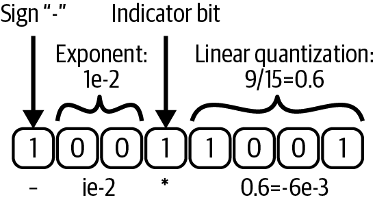
Figure 4-10. Dynamic tree quantization used in 8-bit optimizers: the indicator bit moves dynamically and allows for trade-offs between the fractional and decimal parts of the number (adapted from Dettmers et al., 2022)

The bitsandbytes library provides custom CUDA kernels that leverage dynamic tree quantization in addition to block quantization to provide a more accurate yet performant implementation of a suite of optimizers, including Adam. These implementations (e.g., bnb.optim.Adam8bit) can be swapped for torch.optim.Adam as a one-line change. (You may need a custom compilation of the library, however, based on your version of the NVIDIA runtime.) You will be using this library in the hands-on exercises in Chapters 7 and 9.

A mixed-precision algorithm

Considering the challenges mentioned previously, the summarized algorithm for mixed-precision training is given as follows:

1. Start with a master copy of weights at single precision (fp32).

2. Obtain another half-precision (fp16) copy of the weights.

3. Perform a forward pass using fp16 weights and activations.

4. Scale the resulting loss by the scale factor S.

5. Perform a backward pass using the weights (fp16), activations (fp16), and their gradients (fp32).

6. Scale down the gradients by a factor of S (i.e., multiply by 1/S).

7. Execute additional optional gradient tricks such as gradient clipping, weight decay, etc.

8. Update the gradient statistics (fp16) in the optimizer states.

9. Update the master copy of weights (at fp32).

10. Repeat the iteration loop given by steps 3–9 until convergence.

Memory Tricks for Efficiency

As outlined in Chapter 1, efficiency is a crucial consideration in scaling. In this section we’ll look at a few memory tricks that may be helpful in model development in memory-constrained environments.

Memory layout

The n-dimensional tensors need to be presented in 1D address space in memory. The memory layout defines the storage of n-dimensional tensors, describing how the tensors will be collapsed into the address space. Row-major and column-major are two commonly used formats to lay out the n-dimensional tensors contiguously in memory. As shown in Figure 4-11, row-major is analogous to the batch (N), channel (C), height (H), and width (W)–based scheme (i.e., NCHW, a.k.a. channels first), while column-major is analogous to the NHWC (channels last) scheme.

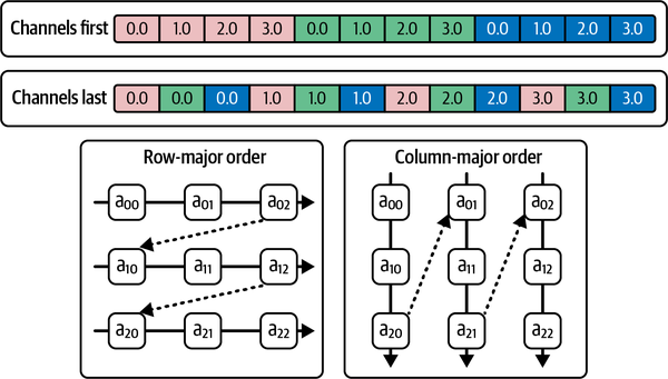
Figure 4-11. Memory layout of channels-first and channels-last tensors

If your operation parallelizes on the channel first, then storing and accessing tensors using the channels-first layout will be more efficient. Other image-based modeling techniques—specifically, convolutions that operate on and exploit spatial correlation of signals in images—access tensors in a more pixel-wise fashion. Thus, for convolution-based techniques, channels last may be a more efficient layout choice. PyTorch supports optionally switching to the channels-last memory layout and supports computation on the same native formats by implementing kernels for a series of operators in channels-last format in addition to the default channels-first format.

Note

Both PyTorch and NVIDIA cuDNN default to the channel-first (NCHW) layout. However, oneDNN and XNNPACK, the libraries PyTorch uses for pure CPU computation, default to channels last (NHWC). Aligning the layout across the entire stack provides more efficient execution of the training loop; otherwise, the access pattern of data becomes suboptimal, incurring a penalty during access of subtensors for relevant operations.

On a CPU, using the channels-last format for convolution-based networks can provide up to a 1.8x time performance gain through appropriate memory access patterns implemented by convolution, pooling, and upsampling layers.¹⁴

To switch the memory layout, you invoke .to(memory_format = torch.channels_last) on either the tensor or the module (to indicate operator preference).

In the second hands-on example in this chapter, you may note images = images.to(memory_format = torch.channels_last) and self.model = self.model.to(memory_format = torch.channels_last) applied when channels last execution is requested. Try this using the following command:

deep-learning-at-scale chapter_4 train-efficient-unet --use-channel-last

On a single A100 SXM 80 GB GPU, using the channels-last format provides about a 10% gain in performance compared to the channels-first configuration.

Likewise, when running the same example on the CPU with the mps backend, using channels last provides a 17% increase in performance over channels first with the same resource settings (a step time of 51.84 s per iteration, down from 62.48 s).

Feature compression

The pervasiveness of memory challenges in deep learning practice is indicated by how commonly GPU OOM errors are faced.¹⁵ The use of data compression (both lossy and lossless) has been explored to reduce the memory footprint of feature maps from the forward pass until they are required again during backward propagation.¹⁶ This technique can reduce the memory requirement by an average of 1.8x; however, it incurs performance overhead from compression/decompression and increased CPU-to-GPU communication. In general, this approach can be useful if there is sparsity or redundancy in the feature maps, but the observed gains will vary highly depending on the nature of the model and data.

Meta and fake tensors

Meta tensors are PyTorch’s underlying mechanism to represent shape and data type without actually allocating memory for storage. PyTorch’s fake tensors are very similar to meta tensors, except that a meta tensor is allocated to an abstract “meta” device whereas fake tensors are allocated to concrete devices (CPUs, GPUs, TPUs, etc.).

A meta tensor is initialized as follows:

meta_layer = torch.nn.Linear(100000, 100000, device = "meta")

We’ll talk more about meta and fake tensors in Chapter 8, where we’ll consider their importance in managing memory in a scaled-up setting.

Optimizer Efficiencies

So far you have looked at several techniques to improve the efficiency of your training runs, including using graph compilation and changing the memory layout and data formats. In this section, you will learn about some gradient tricks to scale out your training on a single host with at most one GPU.

Stochastic gradient descent (SGD)

Early versions of optimizers, such as gradient descent, used the entire training dataset in one step to derive the gradient. But as the dataset size begins to increase, because of memory limitations of computing devices, gradient descent becomes a bottleneck during training. To address this, an approximation technique called stochastic gradient descent (SGD) was devised. With this technique, instead of deriving gradients over the entire sample, the gradients are propagated in batches to arrive at an approximately comparable model.

SGD and other iterative gradient descent techniques are so commonly used these days that one tends to ignore their importance in scaling out large datasets. These techniques are only effective if the batch size is suitable for universal approximation. To develop a model to perform a complex task requiring learning over a highly variant dataset, larger batch sizes are needed to help with universal approximation. The memory budgets on the hardware, however, are limited.

Gradient accumulation

As discussed in the previous section, larger batch sizes are always preferable, as they enable universal approximation (leading to well-generalized models). In scenarios where the compute capacity is restricted but scaling the batch size is desired, gradient accumulation can be used to simulate larger batches.

With gradient accumulation, the standard model training loop, shown here, is transformed to include additional steps of normalizing the loss, accumulating the gradients, and taking the optimization steps every x interval of steps (instead of every step):

# Standard training loop
for epoch in range(...):
    for idx, (inputs, labels) in enumerate(dataloader):
        optimizer.zero_grad()
        # Perform the forward pass
        outputs = model(inputs)
        # Compute loss
        loss = loss_fn(outputs, labels)
        # Perform backpropagation 
        loss.backward()
        # Update the optimizer
        optimizer.step()

The snippet for gradient accumulation follows, where accumulation_step_count indicates the frequency with which the optimization step is taken:

accumulation_step_count = ...

# Training loop with gradient accumulation enabled
for epoch in range(...):
    for idx, (inputs, labels) in enumerate(dataloader):
        optimizer.zero_grad()
        # Perform the forward pass
        outputs = model(inputs)
        # Compute loss 
        loss = loss_fn(outputs, labels)
        # Perform gradient normalization 
        loss = loss / accumulation_step_count
        # Perform backpropagation 
        loss.backward()
        # Update the optimizer
        if ((idx + 1) % accumulation_step_count == 0) \
                    or (idx + 1 == len(dataloader)):
                optimizer.step()

This technique is primarily designed to obtain more accurate models in settings where GPU resources are limited, rather than to provide computation efficiencies.

Gradient checkpointing

More popular optimization techniques used today, such as SGD and Adam, are stateful: they save the statistics of the past gradient values over time (e.g., the exponentially smoothed sum in SGD with momentum and the squared sum in Adam). Some optimizers have higher memory requirements than others. For instance, AdamW saves two states and hence has twice the memory requirements of SGD.

You can check this out by swapping AdamW for SGD in the configure_optimizers call in vision_model.py and observe the memory requirement dropout.

Gradient checkpointing is a technique that aims to be more memory efficient at the expense of computational overhead. If you look at the DAG (discussed in Chapter 2) generated for a Conv2dReLUWithBN, as used in hands-on exercise #2, you may notice that some nodes share the gradient propagation path. Traditionally, gradients for these nodes are saved in memory until all downstream children in the backward direction have been traversed and their respective gradients have been computed. The other extreme of this implementation is to not save the gradients and instead recompute them on demand. If computation latency is not extensive, then this trade-off might provide larger memory capacity to train the model or increase the batch size, for instance. These approaches are the two extreme ends of the spectrum. Gradient checkpointing, a.k.a. activation checkpointing, provides a middle ground: it allows saving gradients at known checkpoints, to find an optimal balance between freeing up memory and reducing redundant compute overhead.

This capability is packaged in PyTorch’s torch.utils.checkpoint.checkpoint module. In Chapter 5, there are hands-on exercises that involve exploring gradient checkpointing.

Patch Gradient Descent

Patch Gradient Descent (PatchGD) is another very interesting technique that can be used to scale the training of gigapixel images that cannot fit into a single GPU (see Figure 4-12).¹⁷ It’s similar to the gradient accumulation technique, except in PatchGD the gradients are accumulated across the various spatial locations of the same image, rather than over independent samples. With this technique, each image is chunked in patches and bundles of patches are passed through the training loop in multiple steps. During these steps, the gradients are accumulated in the corresponding gradient vector until all patches have been passed through.

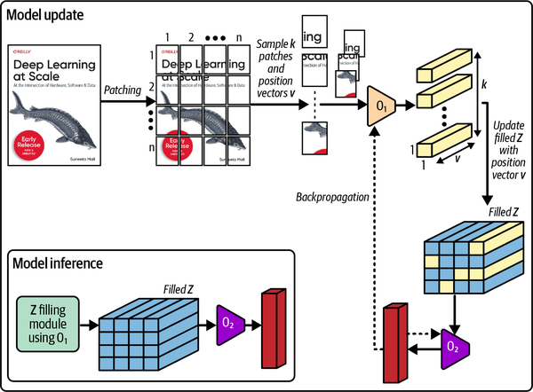
Figure 4-12. The workflow of PatchGD shown over a very large image sample

This technique is only effective for classification-like models where the gradient’s size is much smaller than for models used for more dense tasks, like detections. With PatchGD, the input is chunked, but the gradient is maintained in memory at its full size. Thus, for this trick to work, the estimated gradient vector must fit in memory.

Learning rate and weight decay

The learning rate is another crucial parameter with deep ties to convergence time. As discussed in Chapter 2, with a slower learning rate, it will typically take a lot longer and many more steps to arrive at convergence or global minima. Conversely, a very high learning rate may lead to navigating the loss curvature too fast, resulting in missing out on the global minima and arriving at a suboptimal model. Weight decay can be applied through optimizers as well to enforce regularization (via L2 normalization) to mitigate overfitting. Both learning rate and weight decay influence convergence time.

For this reason, right-sizing the learning rate is a fruitful exercise. Unfortunately, due to its stochastic nature, conducting hyperparameter tuning might be the only solution to optimize the learning rate. In Part II of this book, we will take a deep dive into experimental design and parameter search, and you’ll work through some exercises to tune the model’s parameters.

Model Input Pipeline Tricks

In both of this chapter’s hands-on examples, a very small portion of the compute cycles were used by the model input pipeline (i.e., the DataLoaders). As the volume and data size per sample increases, the increase in computation required to load, uncompress, and read and further transform the dataset could become quite challenging. In Chapter 6, you will learn about training with massive-scale datasets, including techniques to develop efficient DataLoaders to keep GPUs busy and maximize SM utilization. Some of these techniques involve choosing the right compression for your data, scaling out CPU-bound operations with thread and process parallelism (covered in detail in Chapter 3), and moving scalable transformations to the GPU, either via libraries providing GPU-compliant transformations, such as Kornia, or understanding the CPU–GPU memory bandwidth bottlenecks to right-size your inputs. Chapter 7 will feature a hands-on exercise that dives into the details of writing efficient input pipelines.

In the following section, we’ll look at a small example of writing custom CUDA kernels in PyTorch 2.0 using OpenAI Triton.

Writing Custom Kernels in PyTorch 2.0 with Triton

Triton’s programming model is analogous to CUDA programming in that both support SIMD(/T) parallelism. Triton can facilitate the construction of high-performance compute kernels for neural networks using SIMD-style programming paradigms. Its programming model is different than CUDA’s, however, in that the programs—rather than threads—are blocked.

A hands-on example to write a custom kernel for NVIDIA, custom_kernel_example.py, is available in the book’s GitHub repository.

In this code, the kernel multiply_kernel is called on a block of 1,024 elements of the tensors to perform multiplication and store the output in relevant positions. In this example, MultiplyWithAutoGrad implements a function with an automatic differentiation feature. This function can be invoked as follows:

MultiplyWithAutoGrad.apply(
    torch.ones((1999, 1999, 10)).to(device),
    torch.ones((10, 1999, 1999)).to(device)
)

Another emerging PyTorch compiler backend, Hidet, allows more fine-grained compiler optimization than Triton because of its ability to operate at the thread level (unlike Triton, which operates at the block level) and support for additional paradigms like task mapping and fusion to further optimize at the operator and tensor level.¹⁸ This compiler can shave off about 50% of compute time as compared to Triton/max-autotune. It is, however, currently limited to inference only, with training on the roadmap.

Summary

In this chapter, you learned about GPT-2 and EfficientNet as two architectures for two different input formats: text and images. In addition to these hands-on examples, you learned about a variety of techniques to develop models more efficiently. This chapter concludes the first part of the book, focusing on introducing various fundamental techniques required for accelerating and scaling your deep learning model training.

In the next part of this book, you will learn techniques to scale out model training from one to many accelerated devices, using many more hosts connected over the network.

¹ Radford, Alec, Jeffrey Wu, Rewon Child, David Luan, Dario Amodei, and Ilya Sutskever. 2019. “Language Models Are Unsupervised Multitask Learners.” https://paperswithcode.com/paper/language-models-are-unsupervised-multitask; Tan, Mingxing, and Quoc V. Le. 2019. “EfficientNet: Rethinking Model Scaling for Convolutional Neural Networks.” arXiv, May 28, 2019. https://arxiv.org/abs/1905.11946.

² Alammar, Jay. 2019. “The Illustrated GPT-2 (Visualizing Transformer Language Models).” Jay Alammar’s blog, August 12, 2019. https://jalammar.github.io/illustrated-gpt2.

³ Vaswani, Ashish, Noam Shazeer, Niki Parmar, Jakob Uszkoreit, Llion Jones, Aidan N. Gomez, Lukasz Kaiser, and Illia Polosukhin. 2017. “Attention Is All You Need.” arXiv, December 6, 2017. https://arxiv.org/abs/1706.03762.

⁴ Bubeck, Sébastien, Varun Chandrasekaran, Ronen Eldan, Johannes Gehrke, Eric Horvitz, Ece Kamar, Peter Lee, et al. 2023. “Sparks of Artificial General Intelligence: Early Experiments with GPT-4.” arXiv, April 13, 2023. https://arxiv.org/abs/2303.12712.

⁵ Brown, Tom B., Benjamin Mann, Nick Ryder, Melanie Subbiah, Jared Kaplan, Prafulla Dhariwal, Arvind Neelakantan, et al. 2020. “Language Models Are Few-Shot Learners.” arXiv, May 28, 2020. https://arxiv.org/abs/2005.14165.

⁶ Dosovitskiy, Alexey, Lucas Beyer, Alexander Kolesnikov, Dirk Weissenborn, Xiaohua Zhai, Thomas Unterthiner, Mostafa Dehghani, et al. 2021. “An Image Is Worth 16x16 Words: Transformers for Image Recognition at Scale.” arXiv, June 3, 2021. https://arxiv.org/abs/2010.11929.

⁷ Cheng, Bowen, Ishan Misra, Alexander G. Schwing, Alexander Kirillov, Rohit Girdhar. 2022. “Masked-Attention Mask Transformer for Universal Image Segmentation.” arXiv, June 15, 2022. https://arxiv.org/abs/2112.01527.

⁸ Tan and Le, “EfficientNet: Rethinking Model Scaling for Convolutional Neural Networks,” https://arxiv.org/abs/1905.11946; Ronneberger, Olaf, Philipp Fischer, and Thomas Brox. 2015. “U-Net: Convolutional Networks for Biomedical Image Segmentation.” arXiv, May 18, 2015. https://arxiv.org/abs/1505.04597.

⁹ LeCun, Y., B. Boser, J.S. Denker, D. Henderson, R.E. Howard, W. Hubbard, and L.D. Jackel. 1989. “Backpropagation Applied to Handwritten Zip Code Recognition.” Neural Computation 1, no. 4: 541–51. https://doi.org/10.1162/neco.1989.1.4.541.

¹⁰ Ng, Andrew. n.d. Stanford CS230 lecture notes. https://cs230.stanford.edu/files/C4M1.pdf.; Skalski, Piotr. “Gentle Dive into Math Behind Convolutional Neural Networks.” Towards Data Science, April 12, 2019. https://oreil.ly/odnbI.

¹¹ Ronneberger et al., “U-Net: Convolutional Networks for Biomedical Image Segmentation,” https://arxiv.org/abs/1505.04597.

¹² Dettmers, Tim, Mike Lewis, Sam Shleifer, and Luke Zettlemoyer. 2022. “8-Bit Optimizers via Block-wise Quantization.” arXiv, June 20, 2022. https://arxiv.org/abs/2110.02861.

¹³ Bengio, Y., P. Simard, and P. Frasconi. 1994. “Learning Long-Term Dependencies with Gradient Descent Is Difficult.” IEEE Transactions on Neural Networks 5, no. 2: 157–66. https://doi.org/10.1109/72.279181.

¹⁴ Ma, Mingfei, Vitaly Fedyunin, and Wei Wei. “Accelerating PyTorch Vision Models with Channels Last on CPU.” PyTorch blog, August 24, 2022. https://oreil.ly/Dr3Tt.

¹⁵ Zhang, Ru, Wencong Xiao, Hongyu Zhang, Yu Liu, Haoxiang Lin, and Mao Yang. 2020. “An Empirical Study on Program Failures of Deep Learning Jobs.” In Proceedings of the ACM/IEEE 42nd International Conference on Software Engineering (ICSE ’20), 1159–70. https://doi.org/10.1145/3377811.3380362.

¹⁶ Jain, Animesh, Amar Phanishayee, Jason Mars, Lingjia Tang, and Gennady Pekhimenko. 2018. “Gist: Efficient Data Encoding for Deep Neural Network Training.” In ACM/IEEE 45th Annual International Symposium on Computer Architecture (ISCA), 776–89. https://doi.org/10.1109/ISCA.2018.00070.

¹⁷ Gupta, Deepak K., Gowreesh Mago, Arnav Chavan, and Dilip K. Prasad. 2023. “Patch Gradient Descent: Training Neural Networks on Very Large Images.” arXiv, January 31, 2023. https://arxiv.org/abs/2301.13817.

¹⁸ Ding, Yaoyao, Cody Hao Yu, Bojian Zheng, Yizhi Liu, Yida Wang, and Gennady Pekhimenko. 2023. “Hidet: Task-Mapping Programming Paradigm for Deep Learning Tensor Programs.” arXiv, February 15, 2023. https://arxiv.org/abs/2210.09603.