Chapter 1. What Nature and History Have Taught Us About Scale
What works at scale may be different from scaling what works.
—Rohini Nilekani
The main goal of this book is to present valuable information to allow you to efficiently and effectively scale your deep learning workload. In this introductory chapter, we’ll consider what it means to scale and how to determine when to start scaling. We’ll dive into the general law of scaling and draw some inspiration from “nature” as the most scalable system. We’ll also look at evolving trends in deep learning and review how innovation across hardware, software, data, and algorithms is converging to power deep learning at scale. Finally, we’ll explore the philosophy behind scaling and review what factors you should consider and what questions you should ask before beginning your scaling journey.
This chapter is front-loaded with philosophy and history. If you prefer technical material, please skip to “Artificial Intelligence: The Evolution of Learnable Systems”.
The Philosophy of Scaling
To scale a system is to grow its ability by adding more resources to it.1 Increasing the capacity of a bridge by adding more lanes to accommodate more vehicles simultaneously is an example of scaling the bridge. Adding more replicas of a service to handle additional simultaneous user requests and increase throughput is an example of scaling the service. Often when people talk about scaling, they start with a high-level goal, intending to scale a scenario or a capability of a higher order. Adding additional lanes to a bridge or adding more replicas of a service may seem like a straightforward goal, but when you start to dissect it and unravel its dependencies and the plan to execute it, you start to notice the challenges and complexities involved in meeting the original objective of scaling.
How can we assess these task- and domain-specific challenges? They’re captured in the general law of scaling.
The General Law of Scaling
The general scaling law, given by y ∝ f(x), defines the scalability of y by its dependency on the variable x. The mathematical relationship given by f(x) is assumed to hold only over a significant interval of x, to outline that scalability by definition is limited and there will be a value of x where the said (scaling) relationship between x and y will break. These values of x will define the limits of scalability of y. The generic expression f(x) indicates the scaling law takes many forms and is very domain/task-specific. The general scaling law also states that two variables may not share any scaling relationship.
For example, the length of an elastic band is proportional to the applied pull and the elasticity of the material. The band’s length grows as more force (pull) is applied. Yet, there comes a time when, upon application of further force, the material reaches its tensile strength and breaks. This is the limit of the material and defines how much the band can scale. Having said that, the band’s elasticity does not share a scaling relationship with some other properties of the material, such as its color.
The history of scaling law is interesting and relevant even today, because it underscores the challenges and limitations that come with scaling.
History of Scaling Law
In the Divine Comedy, the 14th-century writer and philosopher Dante Alighieri gave a poetic depiction of his conception of Hell, describing it as an inverted cone descending in nine concentric rings to the center of the Earth. His description was accompanied by an illustration by Sandro Botticelli known as the Map of Hell. This depiction was taken quite literally, leading to an investigation to measure the diameter of the cone (the so-called Hall of Hell). Galileo Galilei, a young mathematician, used Dante’s poetic verse “Already the Sun was joined to the horizon / Whose meridian circle covers / Jerusalem with its highest point” as the basis for his conclusion that the diameter of the circle of the dome must be equal to the radius of the Earth and that the center of the roof would lie in Jerusalem. Attending to the term “meridian,” Galileo also deduced that the boundary of the roof’s dome would pass through France, at the point where the prime meridian cuts through. Mapping the dome’s tip at Jerusalem and the edge in France, he concluded that the opposite edge would lie in Uzbekistan. Galileo’s deduction of the size of the Hall of Hell resulted in a pretty big structure. He referenced the dome of Florence Cathedral, which is 45.5 meters (149 feet) wide and 1.5 meters (5 feet) thick, and scaled its measurements linearly to deduce that the roof of the hall would have to be 600 km (373 miles) thick in order to support its own weight. His work was well received, landing him a role as a lecturer in mathematics at the University of Pisa.
In an interesting twist, Galileo realized that the structure, at this thickness, would not be very stable. He pronounced that the thickness of the dome would have to increase much faster than the width to maintain the strength of the structure and keep it from collapsing. Galileo’s conclusion was inspired by the study of animal bones, whose thickness, he observed, increases proportionally at a much faster rate than their length. For example, the longest and also strongest bone in humans, the femur, is on average 48 cm (18.9 in) in length and 2.34 cm (0.92 in) in diameter and can support up to 30 times the weight of an adult. The femur of a greyhound, however, measures on average just 19 cm (7.48 in) long and 0.13 cm (0.05 in) thick (see Figure 1-1).2 Between the two species, this is a difference in length of just 2.5x, whereas the human femur is 18x thicker than that of a greyhound! Continuing the comparison, the second largest animal known to have existed in the world (second only to the blue whale), Tyrannosaurus rex, had a femur bone that measured as long as 133 cm (52.4 in), with an approximate thickness of 43 cm (16.9 in).3
Based on his studies, Galileo identified a limitation for the size of animals’ bones, deducing that above a certain length the bones would have to be impossibly thick to maintain the strength needed to support the body. Of course, there are other practical challenges to life on Earth—for example, agility and mobility—that, together with Darwin’s principles, limit the size of animals. I use this natural example to demonstrate the considerations involved in scaling, a topic that is central to this book. This historical context beautifully illustrates that scaling is neither free nor unlimited, and thus the extent of scaling should be considered thoroughly. “Why scale?” is an equally crucial question. Although a human femur bone can support 30 times the weight of an adult, an average human can barely lift weight twice their own. Tiny ants, on the other hand, are known to lift 50 times their weight!
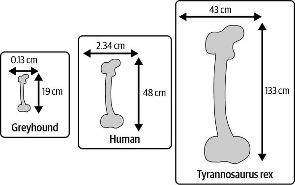
Figure 1-1. The scale of femur bones in three species: greyhound, human, and Tyrannosaurus rex
Ultimately, Galileo’s research led to the general scaling law that forms the basis for many scaling theorems in modern science and engineering. You will read more about some of these laws that are applicable to deep learning scenarios, such as Moore’s law, Dennard scaling, Amdahl’s law, Gunther’s universal scalability law, and the scaling law of language models, in Chapters 3, 5, 8, and 10, respectively.
Scalable Systems
The example discussed in the previous section demonstrates why scaling (increasing the size of an animal, for example) needs to be considered in the context of the entire system (looking at the quality of life of the animal, for example) and its desired abilities (say, to lift heavy weights). It also demonstrates that it is essential to build scalable systems.
Scaling in many ways is about understanding the constraints and dependencies of the system and proportionately scaling the dimensions to achieve the optimal state. Scaling with optimization is more effective than simply scaling. Indeed, everything breaks at scale. Later in this chapter, we’ll talk about considerations for scaling effectively. For now, let’s briefly review nature as a scalable system, and the natural tendency to scale.
Nature as a Scalable System
The surface area of planet Earth totals about 197 million square miles (510 million km2), and it hosts at least 8.7 million unique living species.4 The total population of just one of those 8.7 million species, humans, is estimated to be about 8 billion. As humans, we possess a spectacular ability to digest unlimited data through our visual and auditory senses. What is even more fascinating is that we don’t put any conscious effort into doing so! All combined, we communicate in over 7,100 spoken languages.5 If there is any testament to operating at scale, then the world that surrounds us has got to be it.
With our insatiable appetite for knowledge and exploration of our surroundings and beyond, we are certainly limited by the number of hours in a day. This limitation has resulted in an intense desire to automate the minutiae of our everyday lives and make time to do more within the limits of the day. The challenge with the automation of minutiae is that it’s layered, it’s recursive; once you automate the lowest layer and take it out of the picture, the next layer seemingly becomes the new lowest layer, and you find yourself striving to automate everything.
Let’s take communication as an example. Historically, our ancestors would travel for days or even months to converse in person. The extensive efforts of travel were an obstacle to achieving the objective (conversation). Later, written forms of communication removed the dependency of the primary communicator traveling; messages could be delivered by an intermediary. Over time, the means of propagating written communications across channels also evolved, from carrier pigeons to postal services to Morse code and telegraph. This was followed by the digital era of messages, from faxes and emails to social communication and outreach through internet programs, with everything occurring on the order of milliseconds. We are now in a time of abundance of communication, so much so that we are looking at ways to automatically prioritize what we digest from the plethora of information out there and even considering stochastic approaches to summarizing content to optimize how we use our time. In our quest to eliminate the original obstacles to communication (time and space), we created a new obstacle that requires a new solution. We now find ourselves looking to scale how we communicate, actively exploring the avenues of brain–computer interface and going straight to mind reading.6
Our Visual System: A Biological Inspiration
Scaling is complex. Your limits define how you scale to meet your ambitions. The human visual system is a beautiful example of a scalable system. It’s capable of processing infinite visual signals—literally everything, from the surface of your eyeball to the horizon and everything in between—through a tiny lens with a focal length of about two-thirds of an inch (17 mm). It is simply magnificent that we can do all of that instantly, subconsciously, without any recognizable efforts. Scientists have been studying how the human visual system works for over a hundred years, and while important breakthroughs have been made by the likes of David Hubel and Torsten Weisel,7 we are far from fully understanding the complex mechanism that allows us to perceive our surroundings.
Your brain has about 100 billion neurons. Each neuron is connected to up to 10,000 other neurons, and there are as many as 1,000 trillion synapses passing information between them. Such a complex and scalable system can only thrive if it’s practical and efficient. Your visual system coordinates with about 1015 synapses, yet it consumes only about the amount of energy used by a single LED light bulb (12 watts or so).8 Considering how implicit and subconscious this process is, it’s a good example of minimal input and maximum output—but it does come at the cost of complexity.
As an adaptable information processing system, the level of sophistication the human visual system demonstrates is phenomenal. The cortical cells of the brain are massively parallel. Each cortical cell extracts different information from the same signals. This extracted information is then aggregated and processed, leading to decisions, actions, and experiences. The memories of your experiences are stored in extremely compressed form in the hippocampus. Our biological system is a great example of a parallelized, distributed system designed to handle information efficiently. Scientists and deep learning engineers have drawn a great deal of inspiration from nature and biology, which underscores the importance of efficiency and appreciating considerations of complexity when scaling. This will be the guiding principle through the course of this book as well: I will focus on the principles and techniques of building scalable deep learning systems while considering the complexity and efficiency of such systems.
Many of the advancements in building intelligent (AI) systems have been motivated by the inner workings of biological systems. The fundamental building block of deep learning, the neuron, was inspired by the excitation of biological nervous systems. Similarly, the convolutional neural network (CNN), an efficient technique for intelligently processing computer vision content, was originally inspired by the human visual system. In the following section, you will read about the evolution of learnable systems and review evolving trends in deep learning.
Artificial Intelligence: The Evolution of Learnable Systems
In 1936, Alan Turing presented the theoretical formulation for an imaginary computing device capable of replicating the “states of mind” and symbol-manipulating abilities of a human computer.9 This paper, “On Computable Numbers, with an Application to the Entscheidungsproblem” went on to shape the field of modern computing. Twelve years after Turing laid out his vision of “computing machines,” he outlined many of the core concepts of “intelligent machines,” or “[machines] that can learn from experience.”10 Turing illustrated that by memorizing the current state, considering all possible moves, and choosing the one with the greatest reward and least punishment, computers could play chess. His thoughts and theories were more advanced than the capacity of computational hardware at the time, however, severely limiting the realization of chess-playing computers. His vision of intelligent machines playing chess was not realized until 1997, some 50 years later, when IBM’s Deep Blue beat Garry Kasparov, the then world champion, in a six-game match.
It Takes Four to Tango
In the last decade or so, the early 20th-century vision of realizing intelligent systems has suddenly started to seem much more realistic. This evolution is rooted in innovation in the realms of hardware, software, and data, just as much as learning algorithms. In this section, you will read about the collective progress across these four disciplines and how it has been shaping our progress toward building intelligent systems.
The hardware
IBM’s Deep Blue computer boasted 256 parallel processors; it could examine 200 million possible chess moves per second and look ahead 14 moves. The success of Deep Blue was more attributed to hardware advances than AI techniques, as expressed by Noam Chomsky’s observation that the event was “about as interesting as a bulldozer winning an Olympic weightlifting competition.”
This historical anecdote underlines the importance of computational power in the development of AI and machine learning (ML). Historical data, as shown in Figure 1-2, affirms the intensely growing demand for accelerated computation to power AI development. It is also testament to how the hardware and device industry has caught up to meet the demand for billions of floating-point computations per second.11 This growth has largely been guided by Moore’s law, discussed in Chapter 3, which projects a doubling of the number of transistors (on device) every two years. More transistors allows faster matrix multiplication at the level of electronic circuitry. The increasing complexity of building such powerful computers is evident, as the overcoming of Moore’s law is being observed.12
NVIDIA has been the key organization powering the accelerated compute industry, reaching 1,979 trillion floating-point operations per second (1,979 teraFLOPs) for bfloat16 data types with its Hopper chip. Google has also made significant contributions to powering AI computation with its Tensor Processing Unit (TPU), v4 of which is capable of reaching 275 teraFLOPs (bfloat16). Other AI chips, such as Intel’s Habana, Graphcore’s Intelligent Processing Units (IPUs), and Cerebras’s Wafer Scale Engine (WSE), have also been under active development in the last few years.13 The success (or failure) of many research ideas has been attributed to the availability of suitable hardware, popularly referred to as the hardware lottery.14
The limitations and constraints that come forth as a result of intensive energy use and emission are among key challenges for hardware. Some very interesting projects, like Microsoft’s Natick, are exploring sustainable ways to meet increasing intensive computation demands. You will read more about the hardware aspects of deep learning in Chapters 3 and 5.
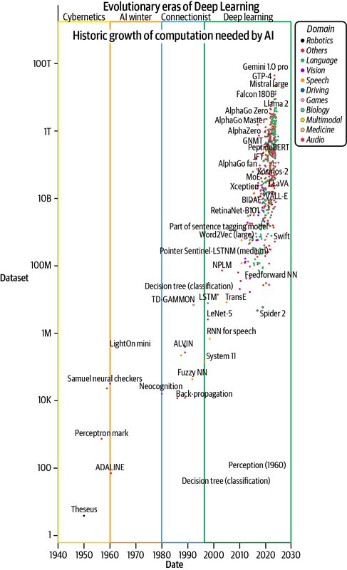
Figure 1-2. Growth of computation needed for developing AI models (plotted using data borrowed from Sevilla et al., 2022)
The data
After hardware, data is the second most critical fuel for deep learning. Tremendous growth in available data and the development of techniques to procure, create, manage, and use it effectively have shaped the success of learnable systems. Deep learning algorithms are data-hungry, but we have been successful in feeding this beast with increasing volumes of data to develop better systems (see Figure 1-3). This is possible because of the exponential growth in digitally created content. For example, in the year 2020 alone, an estimated 64.2e-9 TB (64.2 zettabytes) of data were created—32x more than the 2e-9 TB (2 ZB) created in 2010.15
Note
We’ll talk more about the role of data in deep learning in Chapter 2. A whole range of techniques have been innovated to leverage the volume, variety, veracity, and value of data to develop and scale deep learning models. These techniques are explored under “data-centric AI,” which we’ll discuss in Chapter 10.
Traditionally, the development of intelligent systems started with a highly curated and labeled dataset. More recently, innovative techniques like self-supervised learning have proven quite economical and effective at leveraging a very large corpus of already available unlabeled data—the free-form knowledge that we’ve created throughout history as news articles, books, and various other publications.16 For example, CoCa, a contrastive self-supervised learning model, follows this principle and at the time of writing is the leader in top-1 ImageNet accuracy at 91% (see Figure 1-6 later in this section).17 In addition, social media applications automatically curate vast amounts of labeled multimodal data (e.g., vision data in the form of images with captions/comments and videos with images and audio) that is powering more powerful generalist models (discussed further in Chapters 12 and 13).
Note
Top-N accuracy is a measure of how often the correct label is among the model’s top N predictions. For example, top-1 accuracy indicates how often the model’s prediction exactly matched the expected answer, and top-5 accuracy indicates how often the expected answer was among the model’s top 5 predictions.
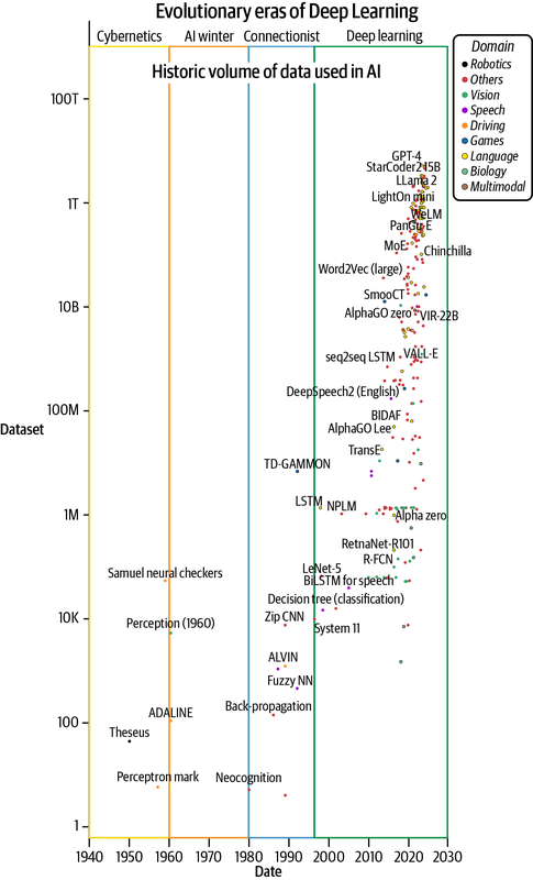
Figure 1-3. Growth in volumes of data used for training AI models (plotted with data from Sevilla et al., 2022)
The software
The software landscape supporting the development of AI solutions has been growing too. During the inception phase, from around the year 2000, only early-stage software frameworks such as MATLAB and the Lua-based Torch were available. This was followed by the formation phase that began around 2012, when machine learning frameworks like Caffe, Chainer, and Theano were developed (see Figure 1-4). It took another four years to reach the maturity phase, which saw stable frameworks like Apache MXNet, TensorFlow, and PyTorch providing more friendly APIs for model development. Attributed to open source communities around the world, working collaboratively to amplify the posture of software tooling for deep learning, we are now in an expansion phase. The expansion phase is defined by the growing ecosystem of software and tools to accelerate the development and productionization of AI software.
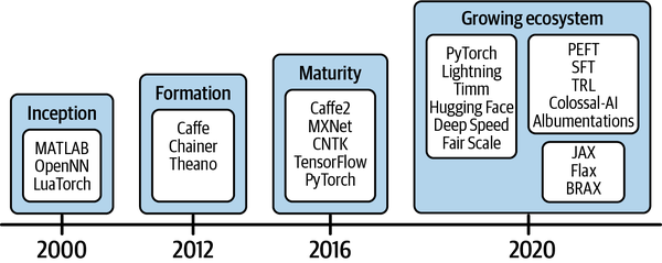
Figure 1-4. The evolutionary phases of software and tooling for deep learning
Community-driven open source development has been key in bringing together the software, algorithms, and people needed for exponential growth. Open source deep learning software development projects (such as PyTorch, JAX, and TensorFlow), foundations such as the Linux Foundation (responsible for PyTorch and its ecosystem), and research sharing forums such as arXiv and Papers with Code have encouraged and enabled contributions from people around the world. The role that open source communities have played in scaling the intelligent system efforts is nothing but heroic.
The (deep learning) algorithms
The vision of learnable intelligent systems started with heuristics-based, rules-driven solutions, which quickly evolved into data-driven stochastic systems. Figure 1-5 charts the evolution and corresponding rise in popularity of deep learning algorithms over time, capturing the progression from the birth of classical machine learning to perceptron-based shallow neural networks to the deeper and denser layers that shaped deep learning today. (For more detailed historical context, see the sidebar “History of Deep Learning”. Note that this is an indicative plot showing the popularity and growth of deep learning; it. It does not represent absolute popularity!) As you can see, the growth in popularity of deep learning has been exponential, but along the way there have been a few lulls—the so-called AI winters—as a result of constraints and limitations that needed to be overcome.
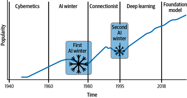
Figure 1-5. The evolution and growth in popularity of deep learning
The second AI winter persisted through 1995. By this point, researchers had realized that to achieve further success with neural networks they needed to find solutions to deal with the following three problems:
- Scaling layers effectively
-
During the Connectionist era, deep learning researchers discovered that effective models for deep learning require a very large number of layers. Simply adding more layers to neural networks was not a viable option, due to overfitting (as outlined by Sepp Hochreiter and Yoshua Bengio et al.).18
- Scaling computation efficiency
-
Unfortunately, the hardware lottery luck was out around this time! For instance, it took three days to train a 9,760-parameter model based on Yann LeCun’s LeNet-5 architecture, proposed in 1989, which had five trainable layers.19 The best computer available at the time was not efficient enough to provide fast feedback, and hardware constraints were throttling development.
- Scaling the input
-
As shown in Figure 1-3, the volume of data used in deep learning experiments barely changed from the 1940s until about 1995. The ability to capture, store, and manage data was also still developing during this time.
Clearly, managing scale is a critical challenge in any deep learning system. The landmark research that accelerated the growth of deep learning was the deep, densely connected belief network developed by Hinton et al. in 2006,20 which has as many parameters as 0.002 mm3 of mouse cortex. This was the first time deep learning had come anywhere close to modeling a biological system, however small. As shown in Figures 1-2 and 1-3, this was also the landmark year when data and hardware gained momentum in their respective growth. Collaborative open source efforts have been drivers of growth too; this is evident from the evolution that followed the release of the ImageNet dataset in 2009, termed the “ImageNet moment.” This dataset, containing over 14 million annotated images of everyday objects in about 20,000 categories, was made available for researchers to compete in the ImageNet Large Scale Visual Recognition Challenge (ILSVRC) and invent algorithms for the scaled-up task.21
Under Hinton’s supervision, in 2017 Alex Krizhevsky produced a solution for the ILSVRC that outperformed the competition by a huge 10.8% margin (at 15.3% top-5 error).22 This work, now popularly known as AlexNet, applied novel distributed training techniques to scale out the development of the solution on two GPUs with very limited memory. Figure 1-6 shows the success trajectory (increasing rate of the top-5 accuracy) of ImageNet since this groundbreaking development.
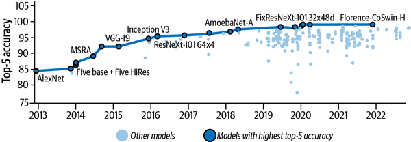
Figure 1-6. Top-5 accuracy of various deep learning models on the ImageNet dataset since the inception of AlexNet (plot based on data obtained from https://oreil.ly/mYfbq)
At around this time, the industry also started to take a serious interest in deep learning and its productionization; solid industry footings positioned it for a cash injection, and venture funding accelerated not just commercialization but also future research. Funds have been flowing into deep learning at a great rate since 2013, when Google’s acquisition of Hinton’s DNNresearch opened the floodgates, making it (as of 2023) a $27 billion industry.23 The abundance of resourcing and support has supercharged the rise of deep learning over the past decade—and with industry support came the interdisciplinary growth that has driven the collective development of scientific aspects of deep learning and algorithms along with everything else that lies at the intersection of hardware, software, and data.
Now that you’re familiar with a little of the history, in the next section we’ll look at current trends in deep learning and see how the ability to scale is influencing ongoing research and industry adaptation.
Evolving Deep Learning Trends
Twenty years after Deep Blue’s success, deep learning has evolved to entirely replace rules-based solutions and is increasingly superseding human-level performance in specific tasks. AlphaGo,24 for instance, reached this level after about four hours of training on a single 44-CPU-core machine with a TPU and can achieve approximate convergence in about nine hours through its novel algorithms and software implementations. It has defeated Stockfish, one of the world’s top chess engines that has won various chess competitions. This enhanced ability to provide better solutions than rule/logic-based software is recognized by the Software 2.0 migration (discussed in more detail in Chapter 2), where traditional software is being made model-driven.
General evolution of deep learning
The application of deep learning in computer vision that began with Yann LeCun’s digit recognition network25 has today scaled to many vision tasks, such as image classification, object detection and segmentation, scene understanding, captioning, etc. These solutions are commonly developed and used around the world today. Efficiency was the key motivation behind the convolutional neural network architecture mentioned earlier in this chapter, and given the voluminous nature of vision data, that has remained a key consideration. CNN-based models like ResNet and EfficientNet have been very successful at vision tasks, reaching a top-1 accuracy of about 90% while carefully applying efficiency and scaling considerations. These models are great for small spatial contexts, but they don’t scale for larger spatial contexts.
Google’s Transformer architecture,26 which pays attention to tokens in long sequences in a parallelized fashion, has been groundbreaking. Requirements to scale vision models for a global context have led to the exploration of the use of Transformer-based architectures. One such example is the Vision Transformer (ViT),27 which tokenizes the images into small chunks and memorizes where these chunks lie in the global image space. For the last few years, most vision research has been driven by the Transformer architecture. CoAtNet, a combination of CNN and Transformer architectures, has 2.44 billion parameters and reaches 90.88% top-1 accuracy on ImageNet tasks. MaxViT, a ViT-based architecture, is close to CoAtNet on the accuracy benchmark but has about five times fewer parameters (475 million).28 Still, scaling the context size of Transformers has remained a challenge due to memory and compute limitations. This has led to interesting and innovative techniques like MEGABYTE and LongViT, which can process very large context sizes (e.g., million-byte sequences or the gigapixel images used in pathology).29 Scaling is not just about parameter count, however; data, energy, and cost economies are critical too.
It was the Transformer architecture that revived innovation in the language processing domain, which had stagnated prior to 2017. Despite suffering from compute inefficiencies (due to quadratic computation in the attention module), this architecture completely revolutionized natural language processing. As shown in Figure 1-7, language models based on this architecture were able to scale their abilities by scaling the number of parameters—a trend referred to as the scaling law of language models.30 OpenAI’s Codex is one such scaled-up model; trained with open source code from GitHub, it is revolutionizing how developers code today. This trend continued until at least mid-2021. What followed in late 2021 was a serious reconsideration of scaling mainly by scaling the number of parameters, and a plateau ensued with a few significant dips caused by models that used considerably lower numbers of parameters but still outperformed their counterparts. Chinchilla is one such model that scales mainly on data volume; despite having 2.5 times fewer parameters, it still outperforms GPT-3. LLaMA, another comparable model from Meta, has also gained popularity and is widely used. This trend can be seen in Figure 1-7, which highlights the model concentration zone around 7B-200B range even though >1T parameter models are being developed.
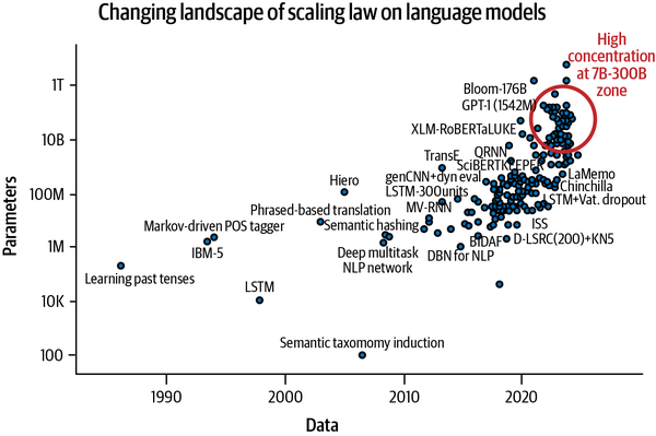
Figure 1-7. The changing landscape of the scaling law of language models (plotted with data from Sevilla et al., 2022)
The scaling law of deep learning models has been encouraging the development of overparameterized models and ever deeper and denser networks.31 This trend is seen across all data modality vision, language, speech, etc. As mentioned earlier, an important innovation at the intersection of data and algorithms is self-supervised model development.32 Together, these developments are supporting the creation of more general-purpose large models that exhibit emerging capabilities, enabling them to perform tasks without being explicitly trained for them. These large models, more commonly known as foundation models, leverage a suite of complex, well-engineered distributed training techniques to efficiently utilize the available resources to produce the best possible models. Another emerging trend is the development of large multimodal models (LMMs) that can work with data from different modalities (such as text, audio, and images), like CLIP and DALL-E, GPT-4, Gemini, and Flamingo. This in turn has led to rapid growth in generative art, with models like Sora, GLIDE, Imagen, and Stability.ai’s Stable Diffusion creating a shakeup within the art industry.33
None of these developments would have been possible without advancements in algorithms, hardware, software, and data. You will read about these developments in Part I. In Part II we’ll look at the details of distributed training, and in Part III we will dive deeper into the efficient and effective development of large-scale models, including foundation models.
Evolution in specialized domains
Aside from general-purpose progress, deep learning has also massively influenced processes and techniques in specialized domains such as the ones discussed in this section.
Math and compute
For centuries, mathematicians believed that the standard matrix multiplication algorithm was the most efficient one. Then, in 1969, Volker Strassen demonstrated another algorithm to be superior. The effort to optimize matrix computation has been ongoing. The overcoming of Moore’s law necessitated exploration of alternative techniques to scale matrix multiplication, leading to approximating multiplication, which yields a 100x speedup but is less practical for scenarios where accuracy matters.34 The most recent discovery, led by DeepMind, identified improvements to Strassen’s algorithm for the first time since its discovery a half-century ago through the use of the deep learning system AlphaTensor.35
Protein folding
Another example of the success of open source and community-driven work is the effort to solve problems in protein folding research by automatically predicting evolutionary protein sequences end to end. AlphaFold, another deep learning system from DeepMind, scaled the protein dataset from 190K empirically derived structures to 0.2B AI-generated protein structures.36 A great example of scale is ProGen2, a 6.4B-parameter model developed using distributed deep learning techniques to scale training across 256 nodes on TPUs.37 The heated competition led to ESMFold, a 15B-parameter model requiring about 2,000 V100 NVIDIA GPUs to develop, that performs six times faster than AlphaFold2 at inference time.38 With these innovations, the protein folding research community basically went from “the protein folding problem currently has no solution” to “deep learning solved it (mostly).”
Simulated world
Deep learning has made quite an impact on virtual reality and physics-guided simulation, even in designing and planning fabrics, and other related industries. The CVPR 2022 keynote “Understanding Visual Appearance from Micron to Global Scale” by Kavita Bala, Dean of Computing and Information Science at Cornell University, is an excellent talk highlighting how deep learning is changing industries all around.
You’ve read a lot about the history and evolution of deep learning in this chapter. In the following section, I will switch the focus to practical considerations and general principles that are essential to scaling. I believe an understanding of these issues is critical before I begin talking about how to scale your deep learning workload, although the guidance I provide here is so generic that it applies not only to deep learning but to scaling any task, engineering or otherwise.
Scale in the Context of Deep Learning
Scaling, in the context of deep learning, is multidimensional, broadly consisting of the following three aspects:
- Generalizability
-
Increasing the ability of models to generalize to diverse tasks or demographics
- Training and development
-
Scaling the model training technique to shorten development time while meeting resource requirements
- Inference
-
Increasing the serviceability of the developed model during serving
All of these are nuanced and require different strategies to scale. This book, however, will focus primarily on the first two; inference (deployment, serving, and servicing) is beyond the scope of the book.
Six Development Considerations
There are six considerations that are crucial to explore when developing a deep learning solution. Let’s take a realistic use case as a basis to explore these considerations to decide when scaling might be necessary and how to prepare for it. I will be using this example throughout this section and often across the book.
Let’s assume that you have built a system that analyzes satellite images to predict if there are any roofs present and, if so, what kinds of roof materials have been used. Let’s also hypothesize that this system has originally been developed for Sydney, Australia. Your model is a vision-based supervised model. So, you have a ground truth dataset representative of roofs and roof materials used in Sydney, and the model has been trained with this dataset. Now, you want to scale your solution to work for any roof in the world!
When you start to decompose this mission, you soon realize that to be able to achieve this goal you’ll need to consider the six aspects outlined in the following sections.
Well-defined problem
For data-driven solutions such as deep learning, it is really important to understand the exact problem one needs to solve and whether you have the right data for that problem.
So, to scale your solution to work for any roof in the world, the problem needs to be defined well. Consider questions like:
-
Are we still just detecting the presence of a roof and the materials used? Or are we expanding to determine the roof style as well (e.g., hip, gable, flat)?
-
How do the materials and shapes of roofs vary across geographies?
-
Are our success criteria uniform, or do we need to trade off sensitivity versus specificity given the circumstances (for certain roofs or specific geographies, for instance)?
-
How are the least and most acceptable error thresholds defined, and what are they? Are there any other success criteria?
These questions are crucial because, for example, if correctly detecting igloo roofs is equally as important as correctly detecting concrete roofs, you may have the added complexity of data imbalance given that concrete roofs are so common but igloos are likely to be underrepresented in your dataset. Geographical nuances, such as Canadian roofs that are often covered in snow, will need to be carefully managed too. This exercise of completely understanding your problem helps you extrapolate the limitations of your system and plan to effectively manage them with your constraints. Scaling is constrained, after all!
Domain knowledge (a.k.a. the constraints)
As discussed previously, scaling for detection of roofs and roof materials necessitates a very good understanding of factors like the following:
-
What defines a roof? Are there certain minimum dimensions? Are only certain shapes or materials recognized?
-
What is included and what is excluded, and why? Do we consider the roof of the shelter at a bus stop a roof? What about pergolas?
-
What are the domain-specific constraints that the solution must follow?
Mapping how roofs and roof materials relate to each other and how geographies constrain the types of roof materials is crucial. For example, rubber roofs have not yet penetrated the Australian market, but rubber is a popular material in Canada because of its ability to protect roofs from extreme weather conditions. Appearance- and material-wise, rubber and shingle roofs are much closer to each other than metal or color bond roofs, for instance. The domain knowledge derived from an extensive understanding of the problem space is often very helpful for building constraints and enforcing validation. For example, with domain knowledge, the model predicting relative probabilities of 0.5 and 0.5 respectively for shingle and rubber roof materials is understandable; however, predicting the same probabilities for tiles and concrete would be less understandable, as the appearance of these materials is quite distinct. Similarly, predicting rubber as the material for Australian roofs will likely be wrong. A good system always understands the user’s expectations—but these can be hard to enforce in a data-driven system such as a deep learning solution. They can more easily be tested and enforced as domain adaptation strategies.
Ground truth
Your dataset is the basis of the knowledge base for your deep learning solution. When planning and building your dataset, you should ask questions like the following:
-
How can we curate the dataset to be representative of roofs around the world?
-
How do we ensure quality and generalization?
Your labeling and data procurement efforts will need to scale accordingly, and this can get really expensive very quickly. As you scale a deep learning system, the ability to quickly iterate on data becomes crucial. Andrej Karpathy, an independent researcher and previous director of AI at Tesla, talks about this in terms of a “data engine”: “Competitive advantage in AI goes not so much to those with data but those with a data engine: iterated data acquisition, re-training, evaluation, deployment, telemetry. And whoever can spin it fastest.”
As you scale, you also start to see interesting odd “real-world” scenarios. Scandinavian sod roofs, for instance, are a very interesting type of region-specific roof. Sod is a less common roof material for people living in many other parts of the world. In areas where it is used, you need to consider issues like how these roofs can be delineated from concrete roofs with artificial turf. How you identify and capture such outliers becomes an interesting challenge too. Having a clear understanding of where you draw the boundaries and what risks you accept is important in scaling your system. You will read more about techniques to handle these challenges in Chapter 10.
Model development
Your goal is to scale the model’s ability to identify roofs and roof materials across the globe. Therefore, your scaling efforts may need to go beyond scaling the dataset (for better representation and generalization) into scaling the capacity of the model and the techniques involved. As discussed previously, if you globalize, your model will need to learn about an increased variety of roof styles and roof material types. If your model is not engineered for this scale, then there may be a risk of underfitting.
You may ask:
-
How do we plan the experiments to arrive at the optimal model for the scaled-up solution?
-
What approach should we adopt to rapidly develop to accelerate the buildup?
-
How can we improvise with our training methodologies so they are most optimal? When do we need distributed training? What efficient training strategies are relevant for our use case?
-
Should we develop with all the data, or use data-centric techniques like sampling and augmentations to accelerate development?
The plans for model evaluation require similar considerations as well, as do structuring the codebase and planning and writing automation tests around model development to support fast and reliable iteration. You will read about scaling model development and training techniques throughout the book, with an explicit focus on experiment planning in Chapter 11.
Deployment
Scaling a system to reach across the globe requires scale and sophistication in deployment strategies as well. While deployment is beyond the scope of this book, I recommend considering the deployment circumstances from the early development stages.
Here are some questions you should consider:
-
What limitations will our deployable environment have?
-
Can we get enough compute and provide the desired latency without compromising the serviceability of user requests for the techniques we’re targeting?
-
How do we get quality metrics from deployed environments for support purposes?
-
How do we optimize the model for various hardware before it’s deployed?
-
Will our choice of tooling support this?
The speed of data processing and the forward pass of the model have direct implications on the serviceability of the system. The warmup and bootstrap lag in surfacing model services directly impacts the scalability strategies the services need to adopt for suitable uptime. This is important data to share as input to the planning of model development.
Feedback
Feedback is crucial for improvement, and there’s no better feedback than direct real-time feedback, straight from your users. A great example of feedback collection is GitHub Copilot. Copilot collects feedback several times after code suggestions are made to gather accurate metrics on the usefulness of the provided suggestions, if the suggestions are still being used, and if so with what level of edits. This is a great opportunity to create a data engine.
As scale increases, the importance of feedback and support systems increases too. In essence, when thinking about feedback, the questions you should be asking are:
-
How are we going to gather feedback from the users to continually improve our system?
-
Can we automate the feedback collection? How can we integrate it with the model development workflow to realize a data engine–like setup?
The feedback needs actioning; otherwise, the feedback system is pointless. In the context of a data engine, measuring the gaps and continually iterating to close these gaps provides significant advantages when building any data-driven system, such as a deep learning solution. This is where the competitive advantage lies.
Scaling Considerations
Scaling is complicated. The mythical “embarrassingly parallel workload” where little or no effort is required to divide and parallelize tasks does not actually exist. For instance, graphics processing units (GPUs) are marketed as embarrassingly parallel devices for matrix computations, but their processing capacity is throttled by their memory bandwidth, limiting the practical computation throughput (see Chapter 3). As discussed earlier, the real challenge of scaling lies in understanding the limitations of subsystems and working with them to scale the entire system.
This section discusses the questions you should be asking before attempting to scale, and the framework for scaling.
Questions to ask before scaling
The proverbial saying “All roads lead to Rome” applies in scaling as well. Often, there may be many ways to achieve the desired scale. The goal should be taking the most optimal route.
For example, to halve the latency of your training process, you may need to scale. You could:
-
Scale your hardware by getting beefier computing devices.
-
Scale your training process by using distributed training.
-
Reduce the computation budget of your process or program at the expense of accuracy/precision.
-
Optimize the input, e.g., by compressing the dataset using data distillation (discussed in Chapter 10).
If you’re financially constrained and unable to fund more or beefier devices, then the optimal route is likely to be option 3 or 4. If you can’t compromise on precision, then by elimination option 4 is the most optimal one. Otherwise, option 3 may be the lowest-hanging fruit to shave the latency.
The topics discussed earlier in this chapter can be distilled into the following set of questions that it’s critical to ask before commencing your scaling efforts. Answering these questions will help you define your options and allow you to scale more effectively:
-
What are we scaling?
-
How will we measure success?
-
Do we really need to scale?
-
What are the ripple effects (i.e., downstream implications)?
-
What are the constraints?
-
How will we scale?
-
Is our scaling technique optimal?
Considering these questions will not only force you to ensure that the scope and limits of scaling are well understood, but also ensure that you have defined good metrics to measure your success. Cassie Kozyrkov, CEO at Data Scientific and previously the chief decision scientist at Google, has an excellent write-up titled “Metric Design for Data Scientists and Business Leaders”39 that outlines the importance of defining metrics first before decisioning. Occam’s razor, the principle of parsimony, highlights the importance of simplicity, but not at the expense of necessity. It is the rule #1 for efficient scaling that you are forced to consider when you ask, “Do we really need to scale?” The following chapters of this book are designed to dive deeply into the approaches and techniques for scaling and help you determine whether your chosen scaling technique is optimal for your use case.
Characteristics of scalable systems
Ian Gorton thoroughly covers the principles of a scalable system, the design patterns used in scaling systems, and the challenges associated with scaling in his book Foundations of Scalable Systems: Designing Distributed Architectures. Gorton’s book is not a prerequisite for this book, but it’s a recommended read if you have some background in software engineering. This section outlines four characteristics of a scalable system that are useful to keep in mind as you prepare to scale your workload.
Reliability
The most important characteristic of a scalable system is reliability. A reliable system rarely fails. In the inopportune moments when it does, it fails predictably, allowing the dependent system and users to gracefully cope with said failure. In other words, a reliable system is capable of coping with (infrequent) failures and recovering from failure scenarios gracefully. Here’s an example: all 224.641e+18 FLOPs that you have performed so far were lost when, due to a network fault, training came to a halt after running for two months using 500 A100 GPU nodes. When the system comes back up, are you able to resume from the last completed computed state and recover gracefully? A reliable system will be able to cope with this failure and gracefully recover.
The commonly known metrics to define a reliable system are as follows:
- Recovery point objective (RPO)
-
RPO is defined as how far back you can go to recover the data after a failure. For example, with checkpointing, the interval you decide on—the frequency with which you store the intermittent weights and training states (optimizers, etc.)—will define your RPO. This might be set in terms of the number of steps or epochs.
- Recovery time objective (RTO)
-
RTO is defined as how long it takes to recover and get back to the state from right before the crash.
- Downtime rate
-
Downtime rate is the percentage of time for which the system is observed to be unavailable or unresponsive.
Availability
Availability defines the likelihood that a system is operational and functional. The gold standard for highly available systems is five nines—i.e., the system is available and functional 99.999% of the time. Managing the availability of a deep learning–based system to five nines is an involved process. TikTok, the small-form video sharing procrastination service by ByteDance Ltd, has been internationally operational since 2017. In five years, it scaled its user content personalization services across 150 countries, hosting over 1 billion users. The system architecture, called Monolith,40 combines online and offline learning to serve user-relevant content, creating sticky users by using click-through rate prediction techniques (DeepFM) and running at scale. While overall availability of TikTok is high, it has faced outage situations on occasions (up to five hours of outage).
Adaptability
Adaptability speaks to how resilient a system is in meeting the growing scaling demands. Are you able to scale the training over the number of available GPUs? How able is the training code to cope with failures like losing a node while training? These are some of the considerations that fall in the purview of adaptability. Some easily solved software engineering challenges surface as incredibly tough problems in the deep learning space.
Performance
Performance is defined in many ways, especially for deep learning–based systems. On the one hand, you have metrics that indicate how good the stochasticity of your deep learning system is and whether it meets the desired standard. On the other hand, you have technical metrics for how well the system is performing—these relate to how many resources it is consuming (RAM, CPU), what the throughput rate is, and so on—that you can monitor when scaling is performed. Ideally, scaling is a favorable event for the stochastic metrics and metrics that drive the expectations and behavior of the system. You do not want the precision of roof detection to fall when you scale your roof detection system across geographies, for instance. Having said that, the technical metrics are expected to align following their respective scaling laws. If you scale the API serving the model to have twice the throughput rate, then you would expect to have the memory requirements change, although you would expect this to have a minimal impact on latency.
Considerations of scalable systems
In a stark reminder of Murphy’s law, the famous saying “Everything breaks at scale!” almost always holds. This should not come as a surprise, because scaling is all about working with the limitations—either to resolve them or to circumvent them. Doing this effectively requires a high level of care and consideration. The following sections touch on some of the factors to keep in mind when designing scalable systems and some commonly useful design patterns for scaling.
Avoiding single points of failure
A single point of failure (SPOF) is a component whose failure can bring the entire system to a halt. Let’s say a model is being trained at scale, across 1,000 A100 GPUs. All these machines are communicating with a distributed data store to read the data needed for training. If this data store fails, it will bring the training to halt; thus, the data store is a single point of failure. Clearly, it’s important to minimize the presence of SPOFs if they can be eradicated.
Designing for high availability
In the previous section, we talked about why availability is an important characteristic of a scalable system. Extending that discussion, all components of a scalable system must be designed to be highly available. High availability is realized through the three Rs: reliability, resilience, and redundancy. This is to say that the components of the system must be designed to be reliable (i.e., to rarely fail and, if they do fail, to do so predictably), resilient (i.e., to gracefully cope with downstream failures without bringing the entire system to halt), and redundant (i.e., to have redundancy baked in so that, in case of a failure, a redundant component can take over without impacting the entire system).
Scaling paradigms
The following three scaling paradigms are commonly used today:
- Horizontal
-
In horizontal scaling, the same system is replicated several times. The replicas are then required to coordinate amongst themselves to provide the same service at scale. Distributed training, in which multiple nodes are added with each node only looking at specific independent parts of a larger dataset, is a very good example of horizontal scaling. This type of scaled training is known as distributed data parallelism; we’ll discuss it further in Chapters 6 and 7.
- Vertical
-
In vertical scaling, the capabilities of the system are scaled by adding more resources to an existing component. Adding more memory cards to increase RAM by 50% is an example of vertical scaling from the node viewpoint. This type of scaled training will be discussed further in Chapters 8 and 9.
- Hybrid
-
In hybrid scaling, both horizontal and vertical scaling techniques are applied to scale across both dimensions. This type of scaled training will be discussed further in Chapters 8 and 9.
Coordination and communication
Coordination and communication are at the heart of any system. Scaling any system creates pressure on the communication backbone used by the system. There are two main communication paradigms:
- Synchronous
-
Synchronous communication occurs in real time, with two or more components sharing information simultaneously. This type of communication is throughput-intensive. As scale (e.g., the number of components) increases, this paradigm of communication very quickly becomes a bottleneck.
- Asynchronous
-
In asynchronous communication, two or more components share information over time. Asynchronous communication provides flexibility and relaxes the communication burden, but it comes at the expense of discontinuity.
Communication and coordination are critical in scaling deep learning systems as well. As an example, stochastic gradient descent (SGD), a technique applied to find the optimal model weights, was originally synchronous. This technique very quickly became a bottleneck in scaling training, leading to the proposal of its asynchronous counterpart, asynchronous SGD (ASGD).41 You will read more about coordination and communication challenges in Chapters 5 and 6.
Caching and intermittent storage
Information retrieval necessitates communication in any system, but the trips to access information from storage are often expensive. This is intensified in deep learning scenarios because the information is spread across compute nodes and GPU devices, making information retrieval involved and expensive. Caching is a very popular technique used to store frequently needed information in inefficient storage to eliminate bottlenecking on this piece of information. Current systems are more limited by memory and communication than by compute power; this is why caching can also be helpful in achieving lower latency.
Process state
Knowing the current state of a process or system is critical to progress to the next stage. How much contextual information a component needs defines whether or not it is stateful: stateless processes and operations don’t require any contextual information at all, whereas stateful processes do. Statelessness simplifies scaling. For example, calculating the dot product of two matrices is a completely stateless operation, as it only requires element-wise operation on indices of the matrix. The statelessness of matrix multiplication enables the so-called embarrassing parallelization of tensor computations. Conversely, gradient accumulation, a deep learning technique used to scale batch size under tight memory constraints, is highly stateful. Using components and techniques that are as stateless as possible reduces complexity of the system and minimizes bottlenecks in scaling.
Graceful recovery and checkpointing
Failures do occur, as is evident from the fact that the gold standard of service availability is five nines (i.e., 99.999% uptime). This acknowledges that even in the most highly available systems, some type of failure will always happen eventually. The sophistication of a scalable system lies in having an efficient pathway to recovery when failure arises, as discussed earlier. Checkpointing is a commonly used technique to preserve intermittent state, storing it as a checkpoint to allow for recovery from the last known good state and maximizing the RPO.
Maintainability and observability
The maintainability of any system is important, because it is directly associated with its continuation. As the complexity of a system increases, as is to be expected when scaling, the cost of maintaining it increases as well. Observability, achieved through monitoring and notification tooling significantly, increases the comfort of working with and maintaining complex systems. Moreover, when failures do occur, identifying and remedying them becomes a much simpler operation, resulting in a shorter RTO.
Scaling effectively
Throughout this chapter, you have gained insight on the importance of scaling effectively. As you have seen, it’s critical to understand what your scale target is, what your limitations are, and what your bottlenecks will be, and to carefully work within your scaling framework to achieve that target.
The old carpentry proverb “measure twice, cut once” has been widely adopted in many domains and has proven its mettle in software development practices. If you’re looking to build quality systems while minimizing the risk of errors and catastrophic failures, it’s very useful to keep this in mind! The same principle applies to deep learning–based systems as well. “Measuring twice and cutting once” is an important strategy for scaling effectively. It provides a much-needed framework to:
-
Know the current benchmarks and highlight known limitations.
-
Test ideas and theories about the solution in a simulated environment and provide fast feedback.
-
Gain confidence in the solution, reducing the risk of errors/accidental gains.
-
Identify subtle, nonobvious bottlenecks early on.
-
Quantify the revised benchmarks with the solution in place.
-
Quickly iterate on strategies for improvement by applying them incrementally.
Efficiency is also about the effective use of available resources. The cost of ineffective deep learning practices is too high, even though letting GPUs “go burrr” has a power law associated with the adrenaline spike it causes in any deep learning practitioner. And that cost is not just limited to money and time; there are environmental and societal effects to consider as well, due to the sheer amount of carbon emissions associated with the energy consumption of these operations and the resulting adverse irreversible climate change impact. Training a large language model such as GPT3 can produce 500 metric tons of carbon dioxide emissions—the equivalent of around 600 flights between London and New York. More carbon-friendly computers like the French supercomputer used for training BLOOM, which is mostly powered by nuclear energy, emit less carbon than traditional GPUs; still, BLOOM is estimated to produce 25 metric tons of carbon dioxide emissions (the equivalent of 30 London–New York flights) during training.42 Techniques like pretraining, few-shot learning, and transfer learning emphasize reducing the training time and repurposing the model’s learnings for other tasks. Pretraining, in particular, lays the foundations for improvements in efficiency through reusability. Contrastive learning implementations such as CoCa, CLIP, and SigLIP are great examples of pretraining at scale achieved via self-supervision.43 Model benchmarks from training with fixed GPU budgets can provide very useful insights for model selection, enabling you to scale efficiently.44
When it comes to climate change, however, limiting carbon emissions at training time is just a feel-good measure—it’s large, but it’s only a one-time expense. Hugging Face estimated that while performing inference, BLOOM emits around 42 lbs (19 kg) of carbon dioxide per day. This is an ongoing expense that will accumulate, amounting to more than the training expenses in about three and a half years.45 These are serious concerns, and the least we can do is make sure we use the resources available to us as efficiently as possible, planning experiments in such a way as to minimize wasted training cycles and using the full capacity of GPUs and CPUs. Through the course of this book, we will explore these concepts and various techniques for developing deep learning models effectively and efficiently.
Summary
According to Forbes, in 2021 76% of enterprises were prioritizing AI.46 McKinsey reports that deep learning accounts for as much as 40% of annual revenue created by analytics and predicts that AI could deliver $13 trillion of additional economic output by 2030.47 Through open sourcing and community participation, AI and deep learning are increasingly being democratized. However, when it comes to scaling, due to the expenses involved, the leverage primarily stays with MAANG (previously FAANG) and organizations with massive funding. Scaling up is one of the biggest challenges ML practitioners.48 This should not come as a surprise, because scaling up any deep learning solution requires not only a thorough understanding of machine learning and software engineering, but also data expertise and hardware knowledge. Building industry-standard scaled-up solutions lies at the intersection of hardware, software, algorithms, and data.
To get you oriented for the rest of the book, this chapter discussed the history and origins of scaling law and the evolution of deep learning. You read about current trends and explored how the growth of deep learning has been driven by advancements in hardware, software, and data as much as the algorithms themselves. You also learned about key considerations to keep in mind when scaling your deep learning solutions and explored the implications of scale in the context of deep learning development. The complexity that comes with scaling is huge and the cost it carries is not inconsequential. One thing that’s certain is that scaling is an adventure, and it’s a lot of fun! I’m looking forward to helping you gain a deeper understanding of scaling deep learning in this book. In the following three chapters, you’ll start by covering the foundational concepts of deep learning and gaining practical insights into the inner workings of the deep learning stack.
1 Bondi, André B. 2000. “Characteristics of Scalability and Their Impact on Performance.” In Proceedings of the Second International Workshop on Software and Performance (WOSP ’00), 195–203. https://doi.org/10.1145/350391.350432.
2 Hutchinson, John R., Karl T. Bates, Julia Molnar, Vivian Allen, and Peter J. Makovicky. 2011. “A Computational Analysis of Limb and Body Dimensions in Tyrannosaurus rex with Implications for Locomotion, Ontogeny, and Growth.” PLoS One 6, no. 10: e26037. https://www.ncbi.nlm.nih.gov/pmc/articles/PMC3192160.
3 Hutchinson et al., “A Computational Analysis,” e26037; Persons, W. Scott IV, Philip J. Currie, and Gregory M. Erickson. 2019. “An Older and Exceptionally Large Adult Specimen of Tyrannosaurus rex.” The Anatomical Record 303, no. 4: 656–72. https://doi.org/10.1002/ar.24118.
4 National Geographic. n.d. “Biodiversity.” Accessed February 9, 2024. https://education.nationalgeographic.org/resource/biodiversity.
5 Ethnologue. n.d. Languages of the World. Accessed February 9, 2024. https://www.ethnologue.com.
6 Fields, R. Douglas. 2020. “Mind Reading and Mind Control Technologies Are Coming.” Observations (blog), March 10, 2020. https://blogs.scientificamerican.com/observations/mind-reading-and-mind-control-technologies-are-coming.
7 Wurtz, Robert H. 2009. “Recounting the Impact of Hubel and Wiesel.” The Journal of Physiology 587: 2817–23. https://doi.org/10.1113%2Fjphysiol.2009.170209.
8 Jorgensen, Timothy J. 2022. “Is the Human Brain a Biological Computer?” Princeton University Press, March 14, 2022. https://press.princeton.edu/ideas/is-the-human-brain-a-biological-computer.
9 Turing, Alan. 1936. “On Computable Numbers, with an Application to the Entscheidungsproblem.” In Proceedings of the London Mathematical Society s2-43, 544–46. https://doi.org/10.1112/plms/s2-43.6.544.
10 Turing, Alan. 1948. “Intelligent Machinery.” Report for National Physical Laboratory. Reprinted in Mechanical Intelligence: Collected Works of A. M. Turing, vol. 1, edited by D.C. Ince, 107–27. Amsterdam: North Holland, 1992. https://weightagnostic.github.io/papers/turing1948.pdf.
11 Sevilla, Jaime, Lennart Heim, Anson Ho, Tamay Besiroglu, Marius Hobbhahn, and Pablo Villalobos. 2022. “Compute Trends Across Three Eras of Machine Learning.” arXiv, March 9, 2022. https://arxiv.org/abs/2202.05924.
12 Heffernan, Virginia. 2022. “Is Moore’s Law Really Dead?” WIRED, November 22, 2022. https://www.wired.com/story/moores-law-really-dead.
13 Heffernan, “Is Moore’s Law Really Dead?” https://www.wired.com/story/moores-law-really-dead.
14 Hooker, Sara. 2020. “The Hardware Lottery.” arXiv, September 21, 2020. https://arxiv.org/abs/2009.06489.
15 Taylor, Petroc. 2023. “Volume of Data/Information Created, Captured, Copied, and Consumed Worldwide from 2010 to 2020, with Forecasts from 2021 to 2025.” Statista, November 16, 2023. https://www.statista.com/statistics/871513/worldwide-data-created.
16 Chen, Ting, Simon Kornblith, Mohammad Norouzi, and Geoffrey Hinton. 2020. “A Simple Framework for Contrastive Learning of Visual Representations.” arXiv, July 1, 2020. https://arxiv.org/abs/2002.05709.
17 Yu, Jiahui, Zirui Wang, Vijay Vasudevan, Legg Yeung, Mojtaba Seyedhosseini, and Yonghui Wu. 2022. “CoCa: Contrastive Captioners Are Image-Text Foundation Models.” arXiv, June 14, 2022. https://arxiv.org/abs/2205.01917.
18 Hochreiter, S. 1990. “Implementierung und Anwendung eines ‘neuronalen’ Echtzeit-Lernalgorithmus für reaktive Umgebungen.” Institute of Computer Science, Technical University of Munich. https://www.bioinf.jku.at/publications/older/fopra.pdf; Bengio, Y., P. Simard, and P. Frasconi. 1994. “Learning Long-Term Dependencies with Gradient Descent Is Difficult.” IEEE Transactions on Neural Networks 5, no. 2: 157–66. https://doi.org/10.1109/72.279181.
19 LeCun, Y., B. Boser, J.S. Denker, D. Henderson, R.E. Howard, W. Hubbard, and L.D. Jackel. 1989. “Backpropagation Applied to Handwritten Zip Code Recognition.” Neural Computation 1, no. 4: 541–51. https://doi.org/10.1162/neco.1989.1.4.541.
20 Hinton, Geoffrey E., Simon Osindero, and Yee-Whye Teh. 2006. “A Fast Learning Algorithm for Deep Belief Nets.” Neural Computation 18, no. 7: 1527–54. https://doi.org/10.1162/neco.2006.18.7.1527.
21 Deng, Jia, Wei Dong, Richard Socher, Li-Jia Li, Kai Li, and Fei-Fei Li. 2009. “ImageNet: A Large-Scale Hierarchical Image Database.” In Proceedings of IEEE Conference on Computer Vision and Pattern Recognition (CVPR), 248–55. http://dx.doi.org/10.1109/CVPR.2009.5206848.
22 Krizhevsky, Alex, Ilya Sutskever, and Geoffrey E. Hinton. 2012. “ImageNet Classification with Deep Convolutional Neural Networks.” In Advances in Neural Information Processing Systems (NIPS 2012) 25, no. 2. https://papers.nips.cc/paper_files/paper/2012/file/c399862d3b9d6b76c8436e924a68c45b-Paper.pdf.
23 Thomas, Owen. 2013. “Google Has Bought a Startup to Help It Recognize Voices and Objects.” Business Insider, March 13, 2013. https://www.businessinsider.com/google-buys-dnnresearch-2013-3; Saha, Rachana. 2024. “Deep Learning Market Expected to Reach US$127 Billion by 2028.” Analytics Insight, February 19, 2024. https://www.analyticsinsight.net/deep-learning-market-expected-to-reach-us127-billion-by-2028.
24 Silver, David, Thomas Hubert, Julian Schrittwieser, Ioannis Antonoglou, Matthew Lai, Arthur Guez, Marc Lanctot, et al. 2018. “A General Reinforcement Learning Algorithm That Masters Chess, Shogi, and Go Through Self-Play.” Science 362, no. 6419: 1140–1144. https://doi.org/10.1126/science.aar6404.
25 Turing, “Intelligent Machinery,” 107–27.
26 Vaswani, Ashish, Noam Shazeer, Niki Parmar, Jakob Uszkoreit, Llion Jones, Aidan N. Gomez, Lukasz Kaiser, and Illia Polosukhin. 2017. “Attention Is All You Need.” arXiv, December 6, 2017. https://arxiv.org/abs/1706.03762.
27 Dosovitskiy, Alexey, Lucas Beyer, Alexander Kolesnikov, Dirk Weissenborn, Xiaohua Zhai, Thomas Unterthiner, Mostafa Dehghani, et al. 2021. “An Image Is Worth 16x16 Words: Transformers for Image Recognition at Scale.” arXiv, June 3, 2021. https://arxiv.org/abs/2010.11929.
28 Silver et al., “A General Reinforcement Learning Algorithm,” 1140–1144; Tu, Zhengzhong, Hossein Talebi, Han Zhang, Feng Yang, Peyman Milanfar, Alan Bovik, and Yinxiao Li. 2022. MaxViT: Multi-Axis Vision Transformer. arXiv, September 9, 2022. https://arxiv.org/abs/2204.01697.
29 Yu, Lili, Dániel Simig, Colin Flaherty, Armen Aghajanyan, Luke Zettlemoyer, and Mike Lewis. 2023. “MEGABYTE: Predicting Million-Byte Sequences with Multiscale Transformers.” arXiv, May 19, 2023. https://arxiv.org/abs/2305.07185; Wang, Wenhui, Shuming Ma, Hanwen Xu, Naoto Usuyama, Jiayu Ding, Hoifung Poon, and Furu Wei. 2023. “When an Image Is Worth 1,024 x 1,024 Words: A Case Study in Computational Pathology.” arXiv, December 6, 2023. https://arxiv.org/abs/2312.03558.
30 Kaplan, Jared, Sam McCandlish, Tom Henighan, Tom B. Brown, Benjamin Chess, Rewon Child, Scott Gray, et al. 2020. “Scaling Laws for Neural Language Models.” arXiv, January 23, 2020. https://arxiv.org/abs/2001.08361.
31 Kaplan et al., “Scaling Laws for Neural Language Models,” https://arxiv.org/abs/2001.08361
32 Gorton, Ian. 2022. Foundations of Scalable Systems: Designing Distributed Architectures. Sebastopol, CA: O’Reilly Media.
33 Heikkilä, Melissa. 2022. “Inside a Radical New Project to Democratize AI.” MIT Technology Review, July 12, 2022. https://www.technologyreview.com/2022/07/12/1055817/inside-a-radical-new-project-to-democratize-ai/amp.
34 Blalock, Davis, and John Guttag. 2021. “Multiplying Matrices Without Multiplying.” arXiv, June 21, 2021. https://arxiv.org/abs/2106.10860.
35 Fawzi, Alhussein, Matej Balog, Aja Huang, Thomas Hubert, Bernardino Romera-Paredes, Mohammadamin Barekatain, Alexander Novikov, et al. 2022. “Discovering Faster Matrix Multiplication Algorithms with Reinforcement Learning.” Nature 610: 47–53. https://doi.org/10.1038/s41586-022-05172-4.
36 Hassabis, Demis. 2022. AlphaFold Reveals the Structure of the Protein Universe. DeepMind blog, July 28, 2022. https://deepmind.google/discover/blog/alphafold-reveals-the-structure-of-the-protein-universe.
37 Nijkamp, Erik, Jeffrey Ruffolo, Eli N. Weinstein, Nikhil Naik, and Ali Madani. 2022. “ProGen2: Exploring the Boundaries of Protein Language Models.” arXiv, June 27, 2022. https://arxiv.org/abs/2206.13517.
38 Lin, Zeming, Halil Akin, Roshan Rao, Brian Hie, Zhongkai Zhu, Wenting Lu, Nikita Smetanin, et al. 2023. “Evolutionary-Scale Prediction of Atomic-Level Protein Structure with a Language Model.” Science 379, no. 6637: 1123–30. https://doi.org/10.1126/science.ade2574.
39 Kozyrkov, Cassie. 2022. “Metric Design for Data Scientists and Business Leaders.” Towards Data Science, October 23, 2022. https://towardsdatascience.com/metric-design-for-data-scientists-and-business-leaders-b8adaf46c00.
40 Liu, Zhuoran, Leqi Zou, Xuan Zou, Caihua Wang, Biao Zhang, Da Tang, Bolin Zhu, et al. 2022. “Monolith: Real Time Recommendation System With Collisionless Embedding Table.” arXiv, September 27, 2022. https://arxiv.org/abs/2209.07663.
41 Dean, Jeffrey, and Luiz André Barroso. 2013. “The Tail at Scale.” Communications of the ACM 56, no. 2: 74–80. https://doi.org/10.1145/2408776.2408794; Chen, Jianmin, Xinghao Pan, Rajat Monga, Samy Bengio, and Rafal Jozefowicz. 2017. “Revisiting Distributed Synchronous SGD.” arXiv, March 21, 2017. https://arxiv.org/abs/1604.00981.
42 Heikkilä, Melissa. 2022. “Why We Need to Do a Better Job of Measuring AI’s Carbon Footprint.” MIT Technology Review, November 15, 2022. https://www.technologyreview.com/2022/11/15/1063202/why-we-need-to-do-a-better-job-of-measuring-ais-carbon-footprint.
43 Radford, Alec, Jong Wook Kim, Chris Hallacy, Aditya Ramesh, Gabriel Goh, Sandhini Agarwal, Girish Sastry, et al. 2021. “Learning Transferable Visual Models from Natural Language Supervision.” arXiv, February 26, 2021. https://arxiv.org/abs/2103.00020; Zhai, Xiaohua, Basil Mustafa, Alexander Kolesnikov, and Lucas Beyer. 2023. Sigmoid Loss for Language Image Pre-Training. arXiv, September 27, 2023. https://arxiv.org/abs/2303.15343.
44 Geiping, Jonas, and Tom Goldstein. 2022. “Cramming: Training a Language Model on a Single GPU in One Day.” arXiv, December 28, 2022. https://arxiv.org/abs/2212.14034.
45 Heikkilä, “Why We Need to Do a Better Job of Measuring AI’s Carbon Footprint,” https://www.technologyreview.com/2022/11/15/1063202/why-we-need-to-do-a-better-job-of-measuring-ais-carbon-footprint.
46 Columbus, Louis. 2021. “76% of Enterprises Prioritize AI & Machine Learning in 2021 IT Budgets.” Forbes, January 17, 2021. https://www.forbes.com/sites/louiscolumbus/2021/01/17/76-of-enterprises-prioritize-ai--machine-learning-in-2021-it-budgets.
47 Bughin, Jacques, Jeongmin Seong, James Manyika, Michael Chui, and Raoul Joshi. 2018. “Notes from the AI Frontier: Modeling the Impact of AI on the World Economy.” McKinsey Global Institute discussion paper. https://www.mckinsey.com/featured-insights/artificial-intelligence/notes-from-the-ai-frontier-modeling-the-impact-of-ai-on-the-world-economy.
48 Thormundsson, Bergur. 2022. “Challenges Companies Are Facing When Deploying and Using Machine Learning from 2018, 2020 and 2021.” Statista, April 6, 2022. https://www.statista.com/statistics/1111249/machine-learning-challenges.
Get Deep Learning at Scale now with the O’Reilly learning platform.
O’Reilly members experience books, live events, courses curated by job role, and more from O’Reilly and nearly 200 top publishers.

