Data Science on AWS

Chapter 1. Introduction to Data Science on AWS

In this chapter, we discuss the benefits of building data science projects in the cloud. We start by discussing the benefits of cloud computing. Next, we describe a typical machine learning workflow and the common challenges to move our models and applications from the prototyping phase to production. We touch on the overall benefits of developing data science projects on Amazon Web Services (AWS) and introduce the relevant AWS services for each step of the model development workflow. We also share architectural best practices, specifically around operational excellence, security, reliability, performance, and cost optimization.

Benefits of Cloud Computing

Cloud computing enables the on-demand delivery of IT resources via the internet with pay-as-you-go pricing. So instead of buying, owning, and maintaining our own data centers and servers, we can acquire technology such as compute power, storage, databases, and other services on an as-needed basis. Similar to a power company sending electricity instantly when we flip a light switch in our home, the cloud provisions IT resources on-demand with the click of a button or invocation of an API.

“There is no compression algorithm for experience” is a famous quote by Andy Jassy, CEO, Amazon Web Services. The quote expresses the company’s long-standing experience in building reliable, secure, and performant services since 2006.

AWS has been continually expanding its service portfolio to support virtually any cloud workload, including many services and features in the area of artificial intelligence and machine learning. Many of these AI and machine learning services stem from Amazon’s pioneering work in recommender systems, computer vision, speech/text, and neural networks over the past 20 years. A paper from 2003 titled “Amazon.com Recommendations: Item-to-Item Collaborative Filtering” recently won the Institute of Electrical and Electronics Engineers award as a paper that withstood the “test of time.” Let’s review the benefits of cloud computing in the context of data science projects on AWS.

Agility

Cloud computing lets us spin up resources as we need them. This enables us to experiment quickly and frequently. Maybe we want to test a new library to run data-quality checks on our dataset, or speed up model training by leveraging the newest generation of GPU compute resources. We can spin up tens, hundreds, or even thousands of servers in minutes to perform those tasks. If an experiment fails, we can always deprovision those resources without any risk.

Cost Savings

Cloud computing allows us to trade capital expenses for variable expenses. We only pay for what we use with no need for upfront investments in hardware that may become obsolete in a few months. If we spin up compute resources to perform our data-quality checks, data transformations, or model training, we only pay for the time those compute resources are in use. We can achieve further cost savings by leveraging Amazon EC2 Spot Instances for our model training. Spot Instances let us take advantage of unused EC2 capacity in the AWS cloud and come with up to a 90% discount compared to on-demand instances. Reserved Instances and Savings Plans allow us to save money by prepaying for a given amount of time.

Elasticity

Cloud computing enables us to automatically scale our resources up or down to match our application needs. Let’s say we have deployed our data science application to production and our model is serving real-time predictions. We can now automatically scale up the model hosting resources in case we observe a peak in model requests. Similarly, we can automatically scale down the resources when the number of model requests drops. There is no need to overprovision resources to handle peak loads.

Innovate Faster

Cloud computing allows us to innovate faster as we can focus on developing applications that differentiate our business, rather than spending time on the undifferentiated heavy lifting of managing infrastructure. The cloud helps us experiment with new algorithms, frameworks, and hardware in seconds versus months.

Deploy Globally in Minutes

Cloud computing lets us deploy our data science applications globally within minutes. In our global economy, it is important to be close to our customers. AWS has the concept of a Region, which is a physical location around the world where AWS clusters data centers. Each group of logical data centers is called an Availability Zone (AZ). Each AWS Region consists of multiple, isolated, and physically separate AZs within a geographic area. The number of AWS Regions and AZs is continuously growing.

We can leverage the global footprint of AWS Regions and AZs to deploy our data science applications close to our customers, improve application performance with ultra-fast response times, and comply with the data-privacy restrictions of each Region.

Smooth Transition from Prototype to Production

One of the benefits of developing data science projects in the cloud is the smooth transition from prototype to production. We can switch from running model prototyping code in our notebook to running data-quality checks or distributed model training across petabytes of data within minutes. And once we are done, we can deploy our trained models to serve real-time or batch predictions for millions of users across the globe.

Prototyping often happens in single-machine development environments using Jupyter Notebook, NumPy, and pandas. This approach works fine for small data sets. When scaling out to work with large datasets, we will quickly exceed the single machine’s CPU and RAM resources. Also, we may want to use GPUs—or multiple machines—to accelerate our model training. This is usually not possible with a single machine.

The next challenge arises when we want to deploy our model (or application) to production. We also need to ensure our application can handle thousands or millions of concurrent users at global scale.

Production deployment often requires a strong collaboration between various teams including data science, data engineering, application development, and DevOps. And once our application is successfully deployed, we need to continuously monitor and react to model performance and data-quality issues that may arise after the model is pushed to production.

Developing data science projects in the cloud enables us to transition our models smoothly from prototyping to production while removing the need to build out our own physical infrastructure. Managed cloud services provide us with the tools to automate our workflows and deploy models into a scalable and highly performant production environment.

Data Science Pipelines and Workflows

Data science pipelines and workflows involve many complex, multidisciplinary, and iterative steps. Let’s take a typical machine learning model development workflow as an example. We start with data preparation, then move to model training and tuning. Eventually, we deploy our model (or application) into a production environment. Each of those steps consists of several subtasks as shown in Figure 1-1.

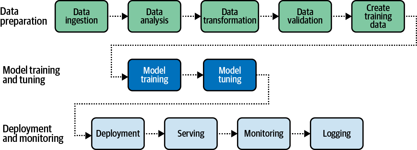
Figure 1-1. A typical machine learning workflow involves many complex, multidisciplinary, and iterative steps.

If we are using AWS, our raw data is likely already in Amazon Simple Storage Service (Amazon S3) and stored as CSV, Apache Parquet, or the equivalent. We can start training models quickly using the Amazon AI or automated machine learning (AutoML) services to establish baseline model performance by pointing directly to our dataset and clicking a single “train” button. We dive deep into the AI Services and AutoML in Chapters 2 and 3.

For more customized machine learning models—the primary focus of this book—we can start the manual data ingestion and exploration phases, including data analysis, data-quality checks, summary statistics, missing values, quantile calculations, data skew analysis, correlation analysis, etc. We dive deep into data ingestion and exploration in Chapters 4 and 5.

We should then define the machine learning problem type—regression, classification, clustering, etc. Once we have identified the problem type, we can select a machine learning algorithm best suited to solve the given problem. Depending on the algorithm we choose, we need to select a subset of our data to train, validate, and test our model. Our raw data usually needs to be transformed into mathematical vectors to enable numerical optimization and model training. For example, we might decide to transform categorical columns into one-hot encoded vectors or convert text-based columns into word-embedding vectors. After we have transformed a subset of the raw data into features, we should split the features into train, validation, and test feature sets to prepare for model training, tuning, and testing. We dive deep into feature selection and transformation in Chapters 5 and 6.

In the model training phase, we pick an algorithm and train our model with our training feature set to verify that our model code and algorithm is suited to solve the given problem. We dive deep into model training in Chapter 7.

In the model tuning phase, we tune the algorithm hyper-parameters and evaluate model performance against the validation feature set. We repeat these steps—adding more data or changing hyper-parameters as needed—until the model achieves the expected results on the test feature set. These results should be in line with our business objective before pushing the model to production. We dive deep into hyper-parameter tuning in Chapter 8.

The final stage—moving from prototyping into production—often presents the biggest challenge to data scientists and machine learning practitioners. We dive deep into model deployment in Chapter 9.

In Chapter 10, we tie everything together into an automated pipeline. In Chapter 11, we perform data analytics and machine learning on streaming data. Chapter 12 summarizes best practices for securing data science in the cloud.

Once we have built every individual step of our machine learning workflow, we can start automating the steps into a single, repeatable machine learning pipeline. When new data lands in S3, our pipeline reruns with the latest data and pushes the latest model into production to serve our applications. There are several workflow orchestration tools and AWS services available to help us build automated machine learning pipelines.

Amazon SageMaker Pipelines

Amazon SageMaker Pipelines are the standard, full-featured, and most complete way to implement AI and machine learning pipelines on Amazon SageMaker. SageMaker Pipelines have integration with SageMaker Feature Store, SageMaker Data Wrangler, SageMaker Processing Jobs, SageMaker Training Jobs, SageMaker Hyper-Parameter Tuning Jobs, SageMaker Model Registry, SageMaker Batch Transform, and SageMaker Model Endpoints, which we discuss throughout the book. We will dive deep into managed SageMaker Pipelines in Chapter 10 along with discussions on how to build pipelines with AWS Step Functions, Kubeflow Pipelines, Apache Airflow, MLflow, TFX, and human-in-the-loop workflows.

AWS Step Functions Data Science SDK

Step Functions, a managed AWS service, is a great option for building complex workflows without having to build and maintain our own infrastructure. We can use the Step Functions Data Science SDK to build machine learning pipelines from Python environments, such as Jupyter Notebook. We will dive deeper into the managed Step Functions for machine learning in Chapter 10.

Kubeflow Pipelines

Kubeflow is a relatively new ecosystem built on Kubernetes that includes an orchestration subsystem called Kubeflow Pipelines. With Kubeflow, we can restart failed pipelines, schedule pipeline runs, analyze training metrics, and track pipeline lineage. We will dive deeper into managing a Kubeflow cluster on Amazon Elastic Kubernetes Service (Amazon EKS) in Chapter 10.

Managed Workflows for Apache Airflow on AWS

Apache Airflow is a very mature and popular option primarily built to orchestrate data engineering and extract-transform-load (ETL) pipelines. We can use Airflow to author workflows as directed acyclic graphs of tasks. The Airflow scheduler executes our tasks on an array of workers while following the specified dependencies. We can visualize pipelines running in production, monitor progress, and troubleshoot issues when needed via the Airflow user interface. We will dive deeper into Amazon Managed Workflows for Apache Airflow (Amazon MWAA) in Chapter 10.

MLflow

MLflow is an open source project that initially focused on experiment tracking but now supports pipelines called MLflow Workflows. We can use MLflow to track experiments with Kubeflow and Apache Airflow workflows as well. MLflow requires us to build and maintain our own Amazon EC2 or Amazon EKS clusters, however. We will discuss MLflow in more detail in Chapter 10.

TensorFlow Extended

TensorFlow Extended (TFX) is an open source collection of Python libraries used within a pipeline orchestrator such as AWS Step Functions, Kubeflow Pipelines, Apache Airflow, or MLflow. TFX is specific to TensorFlow and depends on another open source project, Apache Beam, to scale beyond a single processing node. We will discuss TFX in more detail in Chapter 10.

Human-in-the-Loop Workflows

While AI and machine learning services make our lives easier, humans are far from being obsolete. In fact, the concept of “human-in-the-loop” has emerged as an important cornerstone in many AI/ML workflows. Humans provide important quality assurance for sensitive and regulated models in production.

Amazon Augmented AI (Amazon A2I) is a fully managed service to develop human-in-the-loop workflows that include a clean user interface, role-based access control with AWS Identity and Access Management (IAM), and scalable data storage with S3. Amazon A2I is integrated with many Amazon services including Amazon Rekognition for content moderation and Amazon Textract for form-data extraction. We can also use Amazon A2I with Amazon SageMaker and any of our custom ML models. We will dive deeper into human-in-the-loop workflows in Chapter 10.

MLOps Best Practices

The field of machine learning operations (MLOps) has emerged over the past decade to describe the unique challenges of operating “software plus data” systems like AI and machine learning. With MLOps, we are developing the end-to-end architecture for automated model training, model hosting, and pipeline monitoring. Using a complete MLOps strategy from the beginning, we are building up expertise, reducing human error, de-risking our project, and freeing up time to focus on the hard data science challenges.

We’ve seen MLOps evolve through three different stages of maturity:

MLOps v1.0

Manually build, train, tune, and deploy models

MLOps v2.0

Manually build and orchestrate model pipelines

MLOps v3.0

Automatically run pipelines when new data arrives or code changes from deterministic triggers such as GitOps or when models start to degrade in performance based on statistical triggers such as drift, bias, and explainability divergence

AWS and Amazon SageMaker Pipelines support the complete MLOps strategy, including automated pipeline retraining with both deterministic GitOps triggers as well as statistical triggers such as data drift, model bias, and explainability divergence. We will dive deep into statistical drift, bias, and explainability in Chapters 5, 6, 7, and 9. And we implement continuous and automated pipelines in Chapter 10 with various pipeline orchestration and automation options, including SageMaker Pipelines, AWS Step Functions, Apache Airflow, Kubeflow, and other options including human-in-the-loop workflows. For now, let’s review some best practices for operational excellence, security, reliability, performance efficiency, and cost optimization of MLOps.

Operational Excellence

Here are a few machine-learning-specific best practices that help us build successful data science projects in the cloud:

Data-quality checks

Since all our ML projects start with data, make sure to have access to high-quality datasets and implement repeatable data-quality checks. Poor data quality leads to many failed projects. Stay ahead of these issues early in the pipeline.

Start simple and reuse existing solutions

Start with the simplest solution as there is no need to reinvent the wheel if we don’t need to. There is likely an AI service available to solve our task. Leverage managed services such as Amazon SageMaker that come with a lot of built-in algorithms and pre-trained models.

Define model performance metrics

Map the model performance metrics to business objectives, and continuously monitor these metrics. We should develop a strategy to trigger model invalidations and retrain models when performance degrades.

Track and version everything

Track model development through experiments and lineage tracking. We should also version our datasets, feature-transformation code, hyper-parameters, and trained models.

Select appropriate hardware for both model training and model serving

In many cases, model training has different infrastructure requirements than does model-prediction serving. Select the appropriate resources for each phase.

Continuously monitor deployed models

Detect data drift and model drift—and take appropriate action such as model retraining.

Automate machine learning workflows

Build consistent, automated pipelines to reduce human error and free up time to focus on the hard problems. Pipelines can include human-approval steps for approving models before pushing them to production.

Security

Security and compliance is a shared responsibility between AWS and the customer. AWS ensures the security “of” the cloud, while the customer is responsible for security “in” the cloud.

The most common security considerations for building secure data science projects in the cloud touch the areas of access management, compute and network isolation, encryption, governance, and auditability.

We need deep security and access control capabilities around our data. We should restrict access to data-labeling jobs, data-processing scripts, models, inference endpoints, and batch prediction jobs.

We should also implement a data governance strategy that ensures the integrity, security, and availability of our datasets. Implement and enforce data lineage, which monitors and tracks the data transformations applied to our training data. Ensure data is encrypted at rest and in motion. Also, we should enforce regulatory compliance where needed.

We will discuss best practices to build secure data science and machine learning applications on AWS in more detail in Chapter 12.

Reliability

Reliability refers to the ability of a system to recover from infrastructure or service disruptions, acquire computing resources dynamically to meet demand, and mitigate disruptions such as misconfigurations or transient network issues.

We should automate change tracking and versioning for our training data. This way, we can re-create the exact version of a model in the event of a failure. We will build once and use the model artifacts to deploy the model across multiple AWS accounts and environments.

Performance Efficiency

Performance efficiency refers to the efficient use of computing resources to meet requirements and how to maintain that efficiency as demand changes and technologies evolve.

We should choose the right compute for our machine learning workload. For example, we can leverage GPU-based instances to more efficiently train deep learning models using a larger queue depth, higher arithmetic logic units, and increased register counts.

Know the latency and network bandwidth performance requirements of models, and deploy each model closer to customers, if needed. There are situations where we might want to deploy our models “at the edge” to improve performance or comply with data-privacy regulations. “Deploying at the edge” refers to running the model on the device itself to run the predictions locally. We also want to continuously monitor key performance metrics of our model to spot performance deviations early.

Cost Optimization

We can optimize cost by leveraging different Amazon EC2 instance pricing options. For example, Savings Plans offer significant savings over on-demand instance prices, in exchange for a commitment to use a specific amount of compute power for a given amount of time. Savings Plans are a great choice for known/steady state workloads such as stable inference workloads.

With on-demand instances, we pay for compute capacity by the hour or the second depending on which instances we run. On-demand instances are best for new or stateful spiky workloads such as short-term model training jobs.

Finally, Amazon EC2 Spot Instances allow us to request spare Amazon EC2 compute capacity for up to 90% off the on-demand price. Spot Instances can cover flexible, fault-tolerant workloads such as model training jobs that are not time-sensitive. Figure 1-2 shows the resulting mix of Savings Plans, on-demand instances, and Spot Instances.

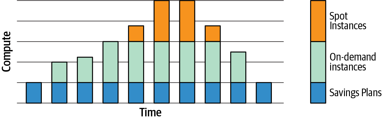
Figure 1-2. Optimize cost by choosing a mix of Savings Plans, on-demand instances, and Spot Instances.

With many of the managed services, we can benefit from the “only pay for what you use” model. For example, with Amazon SageMaker, we only pay for the time our model trains, or we run our automatic model tuning. Start developing models with smaller datasets to iterate more quickly and frugally. Once we have a well-performing model, we can scale up to train with the full dataset. Another important aspect is to right-size the model training and model hosting instances.

Many times, model training benefits from GPU acceleration, but model inference might not need the same acceleration. In fact, most machine learning workloads are actually predictions. While the model may take several hours or days to train, the deployed model likely runs 24 hours a day, 7 days a week across thousands of prediction servers supporting millions of customers. We should decide whether our use case requires a 24 × 7 real-time endpoint or a batch transformation on Spot Instances in the evenings.

Amazon AI Services and AutoML with Amazon SageMaker

We know that data science projects involve many complex, multidisciplinary, and iterative steps. We need access to a machine learning development environment that supports the model prototyping stage and equally provides a smooth transition to prepare our model for production. We will likely want to experiment with various machine learning frameworks and algorithms and develop custom model training and inference code.

Other times, we might want to just use a readily available, pre-trained model to solve a simple task. Or we might want to leverage AutoML techniques to create a first baseline for our project. AWS provides a broad set of services and features for each scenario. Figure 1-3 shows the entire Amazon AI and machine learning stack, including AI services and Amazon SageMaker Autopilot for AutoML.

Figure 1-3. The Amazon AI and machine learning stack.

Amazon AI Services

For many common use cases, such as personalized product recommendations, content moderation, or demand forecasting, we can also use Amazon’s managed AI services with the option to fine-tune on our custom datasets. We can integrate these “1-click” AI services into our applications via simple API calls without much (sometimes no) machine learning experience needed.

The fully managed AWS AI services are the fastest and easiest way to add intelligence to our applications using simple API calls. The AI services offer pre-trained or automatically trained machine learning models for image and video analysis, advanced text and document analysis, personalized recommendations, or demand forecasting.

AI services include Amazon Comprehend for natural language processing, Amazon Rekognition for computer vision, Amazon Personalize for generating product recommendations, Amazon Forecast for demand forecasting, and Amazon CodeGuru for automated source code reviews.

AutoML with SageMaker Autopilot

In another scenario, we might want to automate the repetitive steps of data analysis, data preparation, and model training for simple and well-known machine learning problems. This helps us focus our time on more complex use cases. AWS offers AutoML as part of the Amazon SageMaker service.

Tip

AutoML is not limited to SageMaker. Many of the Amazon AI services perform AutoML to find the best model and hyper-parameters for the given dataset.

“AutoML” commonly refers to the effort of automating the typical steps of a model development workflow that we described earlier. Amazon SageMaker Autopilot is a fully managed service that applies AutoML techniques to our datasets.

SageMaker Autopilot first analyzes our tabular data, identifies the machine learning problem type (i.e., regression, classification) and chooses algorithms (i.e., XGBoost) to solve the problem. It also creates the required data transformation code to preprocess the data for model training. Autopilot then creates a number of diverse machine learning model candidate pipelines representing variations of data transformations and chosen algorithms. It applies the data transformations in a feature engineering step, then trains and tunes each of those model candidates. The result is a ranked list (leaderboard) of the model candidates based on a defined objective metric such as the validation accuracy.

SageMaker Autopilot is an example of transparent AutoML. Autopilot not only shares the data transformation code with us, but it also generates additional Jupyter notebooks that document the results of the data analysis step and the model candidate pipelines to reproduce the model training.

We can leverage SageMaker Autopilot in many scenarios. We can empower more people in our organization to build models, i.e., software developers who might have limited machine learning experience. We can automate model creation for simple-to-solve machine learning problems and focus our time on the new, complex use cases. We can automate the first steps of data analysis and data preparation and then use the result as a baseline to apply our domain knowledge and experience to tweak and further improve the models as needed. The Autopilot-generated model metrics also give us a good baseline for the model quality achievable with the provided dataset. We will dive deep into SageMaker Autopilot in Chapter 3.

Data Ingestion, Exploration, and Preparation in AWS

We will cover data ingestion, exploration, and preparation in Chapters 4, 5, and 6, respectively. But, for now, let’s discuss this portion of the model-development workflow to learn which AWS services and open source tools we can leverage at each step.

Data Ingestion and Data Lakes with Amazon S3 and AWS Lake Formation

Everything starts with data. And if we have seen one consistent trend in recent decades, it’s the continued explosion of data. Data is growing exponentially and is increasingly diverse. Today business success is often closely related to a company’s ability to quickly extract value from their data. There are now more and more people, teams, and applications that need to access and analyze the data. This is why many companies are moving to a highly scalable, available, secure, and flexible data store, often called a data lake.

A data lake is a centralized and secure repository that enables us to store, govern, discover, and share data at any scale. With a data lake, we can run any kind of analytics efficiently and use multiple AWS services without having to transform or move our data.

Data lakes may contain structured relational data as well as semi-structured and unstructured data. We can even ingest real-time data. Data lakes give data science and machine learning teams access to large and diverse datasets to train and deploy more accurate models.

Amazon Simple Storage Service (Amazon S3) is object storage built to store and retrieve any amount of data from anywhere, in any format. We can organize our data with fine-tuned access controls to meet our business and compliance requirements. We will discuss security in depth in Chapter 12. Amazon S3 is designed for 99.999999999% (11 nines) of durability as well as for strong read-after-write consistency. S3 is a popular choice for data lakes in AWS.

We can leverage the AWS Lake Formation service to create our data lake. The service helps collect and catalog data from both databases and object storage. Lake Formation not only moves our data but also cleans, classifies, and secures access to our sensitive data using machine learning algorithms.

We can leverage AWS Glue to automatically discover and profile new data. AWS Glue is a scalable and serverless data catalog and data preparation service. The service consists of an ETL engine, an Apache Hive–compatible data catalog service, and a data transformation and analysis service. We can build data crawlers to periodically detect and catalog new data. AWS Glue DataBrew is a service with an easy-to-use UI that simplifies data ingestion, analysis, visualization, and transformation.

Data Analysis with Amazon Athena, Amazon Redshift, and Amazon QuickSight

Before we start developing any machine learning model, we need to understand the data. In the data analysis step, we explore our data, collect statistics, check for missing values, calculate quantiles, and identify data correlations.

Sometimes we just want to quickly analyze the available data from our development environment and prototype some first model code. Maybe we just quickly want to try out a new algorithm. We call this “ad hoc” exploration and prototyping, where we query parts of our data to get a first understanding of the data schema and data quality for our specific machine learning problem at hand. We then develop model code and ensure it is functionally correct. This ad hoc exploration and prototyping can be done from development environments such as SageMaker Studio, AWS Glue DataBrew, and SageMaker Data Wrangler.

Amazon SageMaker offers us a hosted managed Jupyter environment and an integrated development environment with SageMaker Studio. We can start analyzing data sets directly in our notebook environment with tools such as pandas, a popular Python open source data analysis and manipulation tool. Note that pandas uses in-memory data structures (DataFrames) to hold and manipulate data. As many development environments have constrained memory resources, we need to be careful how much data we pull into the pandas DataFrames.

For data visualizations in our notebook, we can leverage popular open source libraries such as Matplotlib and Seaborn. Matplotlib lets us create static, animated, and interactive visualizations in Python. Seaborn builds on top of Matplotlib and adds support for additional statistical graphics—as well as an easier-to-use programming model. Both data visualization libraries integrate closely with pandas data structures.

The open source AWS Data Wrangler library extends the power of pandas to AWS. AWS Data Wrangler connects pandas DataFrames with AWS services such as Amazon S3, AWS Glue, Amazon Athena, and Amazon Redshift.

AWS Data Wrangler provides optimized Python functions to perform common ETL tasks to load and unload data between data lakes, data warehouses, and databases. After installing AWS Data Wrangler with pip install awswrangler and importing AWS Data Wrangler, we can read our dataset directly from S3 into a pandas DataFrame as shown here:

import awswrangler as wr


# Retrieve the data directly from Amazon S3
df = wr.s3.read_parquet("s3://<BUCKET>/<DATASET>/"))

AWS Data Wrangler also comes with additional memory optimizations, such as reading data in chunks. This is particularly helpful if we need to query large datasets. With chunking enabled, AWS Data Wrangler reads and returns every dataset file in the path as a separate pandas DataFrame. We can also set the chunk size to return the number of rows in a DataFrame equivalent to the numerical value we defined as chunk size. For a full list of capabilities, check the documentation. We will dive deeper into AWS Data Wrangler in Chapter 5.

We can leverage managed services such as Amazon Athena to run interactive SQL queries on the data in S3 from within our notebook. Amazon Athena is a managed, serverless, dynamically scalable distributed SQL query engine designed for fast parallel queries on extremely large datasets. Athena is based on Presto, the popular open source query engine, and requires no maintenance. With Athena, we only pay for the queries we run. And we can query data in its raw form directly in our S3 data lake without additional transformations.

Amazon Athena also leverages the AWS Glue Data Catalog service to store and retrieve the schema metadata needed for our SQL queries. When we define our Athena database and tables, we point to the data location in S3. Athena then stores this table-to-S3 mapping in the AWS Glue Data Catalog. We can use PyAthena, a popular open source library, to query Athena from our Python-based notebooks and scripts. We will dive deeper into Athena, AWS Glue Data Catalog, and PyAthena in Chapters 4 and 5.

Amazon Redshift is a fully managed cloud data warehouse service that allows us to run complex analytic queries against petabytes of structured data. Our queries are distributed and parallelized across multiple nodes. In contrast to relational databases that are optimized to store data in rows and mostly serve transactional applications, Amazon Redshift implements columnar data storage, which is optimized for analytical applications where we are mostly interested in the summary statistics on those columns.

Amazon Redshift also includes Amazon Redshift Spectrum, which allows us to directly execute SQL queries from Amazon Redshift against exabytes of unstructured data in our Amazon S3 data lake without the need to physically move the data. Amazon Redshift Spectrum automatically scales the compute resources needed based on how much data is being received, so queries against Amazon S3 run fast, regardless of the size of our data.

If we need to create dashboard-style visualizations of our data, we can leverage Amazon QuickSight. QuickSight is an easy-to-use, serverless business analytics service to quickly build powerful visualizations. We can create interactive dashboards and reports and securely share them with our coworkers via browsers or mobile devices. QuickSight already comes with an extensive library of visualizations, charts, and tables.

QuickSight implements machine learning and natural language capabilities to help us gain deeper insights from our data. Using ML Insights, we can discover hidden trends and outliers in our data. The feature also enables anyone to run what-if analysis and forecasting, without any machine learning experience needed. We can also build predictive dashboards by connecting QuickSight to our machine learning models built in Amazon SageMaker.

Evaluate Data Quality with AWS Deequ and SageMaker Processing Jobs

We need high-quality data to build high-quality models. Before we create our training dataset, we want to ensure our data meets certain quality constraints. In software development, we run unit tests to ensure our code meets design and quality standards and behaves as expected. Similarly, we can run unit tests on our dataset to ensure the data meets our quality expectations.

AWS Deequ is an open source library built on top of Apache Spark that lets us define unit tests for data and measure data quality in large datasets. Using Deequ unit tests, we can find anomalies and errors early, before the data gets used in model training. Deequ is designed to work with very large datasets (billions of rows). The open source library supports tabular data, i.e., CSV files, database tables, logs, or flattened JSON files. Anything we can fit in a Spark data frame, we can validate with Deequ.

In a later example, we will leverage Deequ to implement data-quality checks on our sample dataset. We will leverage the SageMaker Processing Jobs support for Apache Spark to run our Deequ unit tests at scale. In this setup, we don’t need to provision any Apache Spark cluster ourselves, as SageMaker Processing handles the heavy lifting for us. We can think of this as “serverless” Apache Spark. Once we are in possession of high-quality data, we can now create our training dataset.

Label Training Data with SageMaker Ground Truth

Many data science projects implement supervised learning. In supervised learning, our models learn by example. We first need to collect and evaluate, then provide accurate labels. If there are incorrect labels, our machine learning model will learn from bad examples. This will ultimately lead to inaccurate predictions. SageMaker Ground Truth helps us to efficiently and accurately label data stored in Amazon S3. SageMaker Ground Truth uses a combination of automated and human data labeling.

SageMaker Ground Truth provides pre-built workflows and interfaces for common data labeling tasks. We define the labeling task and assign the labeling job to either a public workforce via Amazon Mechanical Turk or a private workforce, such as our coworkers. We can also leverage third-party data labeling service providers listed on the AWS Marketplace, which are prescreened by Amazon.

SageMaker Ground Truth implements active learning techniques for pre-built workflows. It creates a model to automatically label a subset of the data, based on the labels assigned by the human workforce. As the model continuously learns from the human workforce, the accuracy improves, and less data needs to be sent to the human workforce. Over time and with enough data, the SageMaker Ground Truth active-learning model is able to provide high-quality and automatic annotations that result in lower labeling costs overall. We will dive deeper into SageMaker Ground Truth in Chapter 10.

Data Transformation with AWS Glue DataBrew, SageMaker Data Wrangler, and SageMaker Processing Jobs

Now let’s move on to data transformation. We assume we have our data in an S3 data lake, or S3 bucket. We also gained a solid understanding of our dataset through the data analysis. The next step is now to prepare our data for model training.

Data transformations might include dropping or combining data in our dataset. We might need to convert text data into word embeddings for use with natural language models. Or perhaps we might need to convert data into another format, from numerical to text representation, or vice versa. There are numerous AWS services that could help us achieve this.

AWS Glue DataBrew is a visual data analysis and preparation tool. With 250 built-in transformations, DataBrew can detect anomalies, converting data between standard formats and fixing invalid or missing values. DataBrew can profile our data, calculate summary statistics, and visualize column correlations.

We can also develop custom data transformations at scale with Amazon SageMaker Data Wrangler. SageMaker Data Wrangler offers low-code, UI-driven data transformations. We can read data from various sources, including Amazon S3, Athena, Amazon Redshift, and AWS Lake Formation. SageMaker Data Wrangler comes with pre-configured data transformations similar to AWS DataBrew to convert column types, perform one-hot encoding, and process text fields. SageMaker Data Wrangler supports custom user-defined functions using Apache Spark and even generates code including Python scripts and SageMaker Processing Jobs.

SageMaker Processing Jobs let us run custom data processing code for data transformation, data validation, or model evaluation across data in S3. When we configure the SageMaker Processing Job, we define the resources needed, including instance types and number of instances. SageMaker takes our custom code, copies our data from Amazon S3, and then pulls a Docker container to execute the processing step.

SageMaker offers pre-built container images to run data processing with Apache Spark and scikit-learn. We can also provide a custom container image if needed. SageMaker then spins up the cluster resources we specified for the duration of the job and terminates them when the job has finished. The processing results are written back to an Amazon S3 bucket when the job finishes.

Model Training and Tuning with Amazon SageMaker

Let’s discuss the model training and tuning steps of our model development workflow in more detail and learn which AWS services and open source tools we can leverage.

Train Models with SageMaker Training and Experiments

Amazon SageMaker Training Jobs provide a lot of functionality to support our model training. We can organize, track, and evaluate our individual model training runs with SageMaker Experiments. With SageMaker Debugger, we get transparency into our model training process. Debugger automatically captures real-time metrics during training and provides a visual interface to analyze the debug data. Debugger also profiles and monitors system resource utilization and identifies resource bottlenecks such as overutilized CPUs or GPUs.

With SageMaker training, we simply specify the Amazon S3 location of our data, the algorithm container to execute our model training code, and define the type and number of SageMaker ML instances we need. SageMaker will take care of initializing the resources and run our model training. If instructed, SageMaker spins up a distributed compute cluster. Once the model training completes, SageMaker writes the results to S3 and terminates the ML instances.

SageMaker also supports Managed Spot Training. Managed Spot Training leverages Amazon EC2 Spot Instances to perform model training. Using Spot Instances, we can reduce model training cost up to 90% compared to on-demand instances.

Besides SageMaker Autopilot, we can choose from any of the built-in algorithms that come with Amazon SageMaker or customize the model training by bringing our own model code (script mode) or our own algorithm/framework container.

Built-in Algorithms

SageMaker comes with many built-in algorithms to help machine learning practitioners get started on training and deploying machine learning models quickly. Built-in algorithms require no extra code. We only need to provide the data and any model settings (hyper-parameters) and specify the compute resources. Most of the built-in algorithms also support distributed training out of the box to support large datasets that cannot fit on a single machine.

For supervised learning tasks, we can choose from regression and classification algorithms such as Linear Learner and XGBoost. Factorization Machines are well suited to recommender systems.

For unsupervised learning tasks, such as clustering, dimension reduction, pattern recognition, and anomaly detection, there are additional built-in algorithms available. Such algorithms include Principal Component Analysis (PCA) and K-Means Clustering.

We can also leverage built-in algorithms for text analysis tasks such as text classification and topic modeling. Such algorithms include BlazingText and Neural Topic Model.

For image processing, we will find built-in algorithms for image classification and object detection, including Semantic Segmentation.

Bring Your Own Script (Script Mode)

If we need more flexibility, or there is no built-in solution that works for our use case, we can provide our own model training code. This is often referred to as “script mode.” Script mode lets us focus on our training script, while SageMaker provides highly optimized Docker containers for each of the familiar open source frameworks, such as TensorFlow, PyTorch, Apache MXNet, XGBoost, and scikit-learn. We can add all our needed code dependencies via a requirements file, and SageMaker will take care of running our custom model training code with one of the built-in framework containers, depending on our framework of choice.

Bring Your Own Container

In case neither the built-in algorithms or script mode covers our use case, we can bring our own custom Docker image to host the model training. Docker is a software tool that provides build-time and runtime support for isolated environments called Docker containers.

SageMaker uses Docker images and containers to provide data processing, model training, and prediction serving capabilities.

We can use bring your own container (BYOC) if the package or software we need is not included in a supported framework. This approach gives us unlimited options and the most flexibility, as we can build our own Docker container and install anything we require. Typically, we see people use this option when they have custom security requirements, or want to preinstall libraries into the Docker container to avoid a third-party dependency (i.e., with PyPI, Maven, or Docker Registry).

When using the BYOC option to use our own Docker image, we first need to upload the Docker image to a Docker registry like DockerHub or Amazon Elastic Container Registry (Amazon ECR). We should only choose the BYOC option if we are familiar with developing, maintaining, and supporting custom Docker images with an efficient Docker-image pipeline. Otherwise, we should use the built-in SageMaker containers.

Note

We don’t need to “burn” our code into a Docker image at build time. We can simply point to our code in Amazon S3 from within the Docker image and load the code dynamically when a Docker container is started. This helps avoid unnecessary Docker image builds every time our code changes.

Pre-Built Solutions and Pre-Trained Models with SageMaker JumpStart

SageMaker JumpStart gives us access to pre-built machine learning solutions and pre-trained models from AWS, TensorFlow Hub, and PyTorch Hub. The pre-built solutions cover many common use cases such as fraud detection, predictive maintenance, and demand forecasting. The pre-trained models span natural language processing, object detection, and image classification domains. We can fine-tune the models with our own datasets and deploy them to production in our AWS account with just a few clicks. We will dive deeper into SageMaker JumpStart in Chapter 7.

Tune and Validate Models with SageMaker Hyper-Parameter Tuning

Another important step in developing high-quality models is finding the right model configuration or model hyper-parameters. In contrast to the model parameters that are learned by the algorithm, hyper-parameters control how the algorithm learns the parameters.

Amazon SageMaker comes with automatic model tuning and validating capabilities to find the best performing model hyper-parameters for our model and dataset. We need to define an objective metric to optimize, such as validation accuracy, and the hyper-parameter ranges to explore. SageMaker will then run many model training jobs to explore the hyper-parameter ranges that we specify and evaluate the results against the objective metric to measure success.

There are different strategies to explore hyper-parameter ranges: grid search, random search, and Bayesian optimization are the most common ones. We will dive deeper into SageMaker Hyper-Parameter Tuning in Chapter 8.

Model Deployment with Amazon SageMaker and AWS Lambda Functions

Once we have trained, validated, and optimized our model, we are ready to deploy and monitor our model. There are generally three ways to deploy our models with Amazon SageMaker, depending on our application requirements: SageMaker Endpoints for REST-based predictions, AWS Lambda functions for serverless predictions, and SageMaker Batch Transform for batch predictions.

SageMaker Endpoints

If we need to optimize the model deployment for low-latency, real-time predictions, we can deploy our model using SageMaker hosting services. These services will spin up a SageMaker endpoint to host our model and provide a REST API to serve predictions. We can call the REST API from our applications to receive model predictions. SageMaker model endpoints support auto-scaling to match the current traffic pattern and are deployed across multiple AZs for high availability.

SageMaker Batch Transform

If we need to get predictions for an entire dataset, we can use SageMaker Batch Transform. Batch Transform is optimized for high throughput, without the need for real-time, low-latency predictions. SageMaker will spin up the specified number of resources to perform large-scale, batch predictions on our S3 data. Once the job completes, SageMaker will write the data to S3 and tear down the compute resources.

Serverless Model Deployment with AWS Lambda

Another option to serve our model predictions are AWS Lambda functions for serverless model servers. After training the model with SageMaker, we use an AWS Lambda function that retrieves the model from S3 and serves the predictions. AWS Lambda does have memory and latency limitations, so be sure to test this option at scale before finalizing on this deployment approach.

Streaming Analytics and Machine Learning on AWS

Until now, we assumed that we have all of our data available in a centralized static location, such as our S3-based data lake. In reality, data is continuously streaming from many different sources across the world simultaneously. In many cases, we want to perform real-time analytics and machine learning on this streaming data before it lands in a data lake. A short time to (business) insight is required to gain competitive advances and to react quickly to changing customer and market trends.

Streaming technologies provide us with the tools to collect, process, and analyze data streams in real time. AWS offers a wide range of streaming technology options, including Amazon Kinesis and Amazon Managed Streaming for Apache Kafka (Amazon MSK). We will dive deep into streaming analytics and machine learning in Chapter 11.

Amazon Kinesis Streaming

Amazon Kinesis is a streaming data service, which helps us collect, process, and analyze data in real time. With Kinesis Data Firehose, we can prepare and load real-time data continuously to various destinations including Amazon S3 and Amazon Redshift. With Kinesis Data Analytics, we can process and analyze the data as it arrives. And with Amazon Kinesis Data Streams, we can manage the ingest of data streams for custom applications.

Amazon Managed Streaming for Apache Kafka

Amazon MSK is a streaming data service that manages Apache Kafka infrastructure and operations. Apache Kafka is a popular open source, high-performance, fault-tolerant, and scalable platform for building real-time streaming data pipelines and applications. Using Amazon MSK, we can run our Apache Kafka applications on AWS without the need to manage Apache Kafka clusters ourselves.

Streaming Predictions and Anomaly Detection

In the streaming data chapter, we will focus on analyzing a continuous stream of product review messages that we collect from available online channels. We will run streaming predictions to detect the sentiment of our customers, so we can identify which customers might need high-priority attention.

Next, we run continuous streaming analytics over the incoming review messages to capture the average sentiment per product category. We visualize the continuous average sentiment in a metrics dashboard for the line of business (LOB) owners.

The LOB owners can now detect sentiment trends quickly and take action. We also calculate an anomaly score of the incoming messages to detect anomalies in the data schema or data values. In case of a rising anomaly score, we can alert the application developers in charge to investigate the root cause.

As a last metric, we also calculate a continuous approximate count of the received messages. This number of online messages could be used by the digital marketing team to measure effectiveness of social media campaigns.

AWS Infrastructure and Custom-Built Hardware

A key benefit of cloud computing is the ability to try infrastructure options that specifically match our workload. AWS provides many options for high-performance compute, networking, and storage infrastructure for our data science projects, as Figure 1-4 shows. Let’s see each of these options, which we will reference throughout.

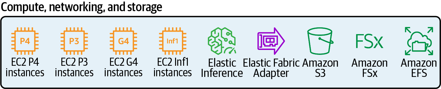
Figure 1-4. AWS infrastructure options for data science and machine learning projects.

SageMaker Compute Instance Types

AWS allows us to choose from a diverse set of instance types depending on our workload. Following is a list of instance types commonly used for data science use cases:

T instance type

General-purpose, burstable-performance instances when we don’t need consistently high levels of CPU but benefit from having fast CPUs when we need them

M instance type

General-purpose instances with a good balance of compute, memory, and network bandwidth

C instance type

Compute-optimized instances ideal for compute-bound workloads with high-CPU requirements

R instance type

Memory-optimized instances optimized for workloads that benefit from storing large datasets in memory such as Apache Spark

P, G, Inferentia, and Trainium instance types

High-performance compute instances with hardware accelerators or coprocessors such as GPUs or Amazon custom-built hardware such as AWS Inferentia for inference and AWS Trainium for training workloads

Amazon Elastic Inference Accelerator

Network-attached coprocessors used by other instance types when additional compute power is needed for specific workloads, such as batch transformations and inference

GPUs and Amazon Custom-Built Compute Hardware

Similar to how Amazon S3 provides storage in the cloud, Amazon Elastic Compute Cloud (Amazon EC2) provides compute resources. We can choose from over 350 instances for our business needs and workload. AWS also offers a choice of Intel, AMD, and ARM-based processors. The hardware-accelerated P4, P3, and G4 instance types are a popular choice for high-performance, GPU-based model training. Amazon also provides custom-build hardware optimized for both model training and inference.

P4d instances consist of eight NVIDIA A100 Tensor Core GPUs with 400 Gbps instance networking and support for Elastic Fabric Adapter (EFA) with NVIDIA GPUDirect RDMA (remote direct memory access). P4d instances are deployed in hyperscale clusters called Amazon EC2 UltraClusters that provide supercomputer-class performance for everyday ML developers, researchers, and data scientists. Each EC2 UltraCluster of P4d instances gives us access to more than 4,000 NVIDIA A100 GPUs, petabit-scale nonblocking networking, and high-throughput/low-latency storage via Amazon FSx for Lustre.

P3 instances consist of up to eight NVIDIA V100 Tensor Core GPUs and deliver up to 100 Gbps of networking throughput. P3 instances deliver up to one petaflop of mixed-precision performance per instance. P3dn.24xlarge instances also support EFA.

The G4 instances are a great option for cost-sensitive, small-scale training or inference workloads. G4 instances consist of NVIDIA T4 GPUs with up to 100 Gbps of networking throughput and up to 1.8 TB of local NVMe storage.

AWS also offers custom-built silicon for machine learning training with the AWS Trainium chip and for inference workloads with the AWS Inferentia chip. Both AWS Trainium and AWS Inferentia aim at increasing machine learning performance and reducing infrastructure cost.

AWS Trainium has been optimized for deep learning training workloads, including image classification, semantic search, translation, voice recognition, natural language processing, and recommendation engines.

AWS Inferentia processors support many popular machine learning models, including single-shot detectors and ResNet for computer vision—as well as Transformers and BERT for natural language processing.

AWS Inferentia is available via the Amazon EC2 Inf1 instances. We can choose between 1 and 16 AWS Inferentia processors per Inf1 instance, which deliver up to 2,000 tera operations per second. We can use the AWS Neuron SDK to compile our TensorFlow, PyTorch, or Apache MXNet models to run on Inf1 instances.

Inf1 instances can help to reduce our inference cost, with up to 45% lower cost per inference and 30% higher throughput compared to Amazon EC2 G4 instances. Table 1-1 shows some instance-type options to use for model inference, including Amazon custom-built Inferentia chip, CPUs, and GPUs.

Table 1-1. EC2 instance options for model inference

Model characteristics	EC2 Inf1	EC2 C5	EC2 G4
Requires low latency and high throughput at low cost	X
Low sensitivity to latency and throughput		X
Requires NVIDIA’s CUDA, CuDNN or TensorRT libraries			X

Amazon Elastic Inference is another option to leverage accelerated compute for model inference. Elastic Inference allows us to attach a fraction of GPU acceleration to any Amazon EC2 (CPU-based) instance type. Using Elastic Inference, we can decouple the instance choice for model inference from the amount of inference acceleration.

Choosing Elastic Inference over Inf1 might make sense if we need different instance characteristics than those offered with Inf1 instances or if our performance requirements are lower than what the smallest Inf1 instance provides.

Elastic Inference scales from single-precision TFLOPS (trillion floating point operations per second) up to 32 mixed-precision TFLOPS of inference acceleration.

Graviton processors are AWS custom-built ARM processors. The CPUs leverage 64-bit Arm Neoverse cores and custom silicon designed by AWS using advanced 7 nm manufacturing technology. ARM-based instances can offer an attractive price-performance ratio for many workloads running in Amazon EC2.

The first generation of Graviton processors are offered with Amazon EC2 A1 instances. Graviton2 processors deliver 7x more performance, 4x more compute cores, 5x faster memory, and 2x larger caches compared to the first generation. We can find the Graviton2 processor in Amazon EC2 T4g, M6g, C6g, and R6g instances.

The AWS Graviton2 processors provide enhanced performance for video encoding workloads, hardware acceleration for compression workloads, and support for machine learning predictions.

GPU-Optimized Networking and Custom-Built Hardware

AWS offers advanced networking solutions that can help us to efficiently run distributed model training and scale-out inference.

The Amazon EFA is a network interface for Amazon EC2 instances that optimizes internode communications at scale. EFA uses a custom-built OS bypass hardware interface that enhances the performance of internode communications. If we are using the NVIDIA Collective Communications Library for model training, we can scale to thousands of GPUs using EFA.

We can combine the setup with up to 400 Gbps network bandwidth per instance and the NVIDIA GPUDirect RDMA for low-latency, GPU-to-GPU communication between instances. This gives us the performance of on-premises GPU clusters with the on-demand elasticity and flexibility of the cloud.

Storage Options Optimized for Large-Scale Model Training

We already learned about the benefits of building our data lake on Amazon S3. If we need faster storage access for distributed model training, we can use Amazon FSx for Lustre.

Amazon FSx for Lustre offers the open source Lustre filesystem as a fully managed service. Lustre is a high-performance filesystem, offering submillisecond latencies, up to hundreds of gigabytes per second of throughput, and millions of IOPS.

We can link FSx for Lustre filesystems with Amazon S3 buckets. This allows us to access and process data through the FSx filesystem and from Amazon S3. Using FSx for Lustre, we can set up our model training compute instances to access the same set of data through high-performance shared storage.

Amazon Elastic File System (Amazon EFS) is another file storage service that provides a filesystem interface for up to thousands of Amazon EC2 instances. The filesystem interface offers standard operating system file I/O APIs and enables filesystem access semantics, such as strong consistency and file locking.

Reduce Cost with Tags, Budgets, and Alerts

Throughout the book, we provide tips on how to reduce cost for data science projects with the Amazon AI and machine learning stack. Overall, we should always tag our resources with the name of the business unit, application, environment, and user. We should use tags that provide visibility into where our money is spent. In addition to the AWS built-in cost-allocation tags, we can provide our own user-defined allocation tags specific to our domain. AWS Budgets help us create alerts when cost is approaching—or exceeding—a given threshold.

Summary

In this chapter, we discussed the benefits of developing data science projects in the cloud, with a specific focus on AWS. We showed how to quickly add intelligence to our applications leveraging the Amazon AI and machine learning stack. We introduced the concept of AutoML and explained how SageMaker Autopilot offers a transparent approach to AutoML. We then discussed a typical machine learning workflow in the cloud and introduced the relevant AWS services that assist in each step of the workflow. We provided an overview of available workflow orchestration tools to build and automate machine learning pipelines. We described how to run streaming analytics and machine learning over real-time data. We finished this chapter with an overview of AWS infrastructure options to leverage in our data science projects.

In Chapter 2, we will discuss prominent data science use cases across industries such as media, advertising, IoT, and manufacturing.