Chapter 4. Ingest Data into the Cloud
In this chapter, we will show how to ingest data into the cloud. For that purpose, we will look at a typical scenario in which an application writes files into an Amazon S3 data lake, which in turn needs to be accessed by the ML engineering/data science team as well as the business intelligence/data analyst team, as shown in Figure 4-1.

Figure 4-1. An application writes data into our S3 data lake for the data science, machine learning engineering, and business intelligence teams.
Amazon Simple Storage Service (Amazon S3) is fully managed object storage that offers extreme durability, high availability, and infinite data scalability at a very low cost. Hence, it is the perfect foundation for data lakes, training datasets, and models. We will learn more about the advantages of building data lakes on Amazon S3 in the next section.
Let’s assume our application continually captures data (i.e., customer interactions on our website, product review messages) and writes the data to S3 in the tab-separated values (TSV) file format.
As a data scientist or machine learning engineer, we want to quickly explore raw datasets. We will introduce Amazon Athena and show how to leverage Athena as an interactive query service to analyze data in S3 using standard SQL, without moving the data. In the first step, we will register the TSV data in our S3 bucket with Athena and then run some ad hoc queries on the dataset. We will also show how to easily convert the TSV data into the more query-optimized, columnar file format Apache Parquet.
Our business intelligence team might also want to have a subset of the data in a data warehouse, which they can then transform and query with standard SQL clients to create reports and visualize trends. We will introduce Amazon Redshift, a fully managed data warehouse service, and show how to insert TSV data into Amazon Redshift, as well as combine the data warehouse queries with the less frequently accessed data that’s still in our S3 data lake via Amazon Redshift Spectrum. Our business intelligence team can also use Amazon Redshift’s data lake export functionality to unload (transformed, enriched) data back into our S3 data lake in Parquet file format.
We will conclude this chapter with some tips and tricks for increasing performance using compression algorithms and reducing cost by leveraging S3 Intelligent-Tiering. In Chapter 12, we will dive deep into securing datasets, tracking data access, encrypting data at rest, and encrypting data in transit.
Data Lakes
In Chapter 3, we discussed the democratization of artificial intelligence and data science over the last few years, the explosion of data, and how cloud services provide the infrastructure agility to store and process data of any amount.
Yet, in order to use all this data efficiently, companies are tasked to break down existing data silos and find ways to analyze very diverse datasets, dealing with both structured and unstructured data while ensuring the highest standards of data governance, data security, and compliance with privacy regulations. These (big) data challenges set the stage for data lakes.
One of the biggest advantages of data lakes is that we don’t need to predefine any schemas. We can store our raw data at scale and then decide later in which ways we need to process and analyze it. Data lakes may contain structured, semistructured, and unstructured data. Figure 4-2 shows the centralized and secure data lake repository that enables us to store, govern, discover, and share data at any scale—even in real time.
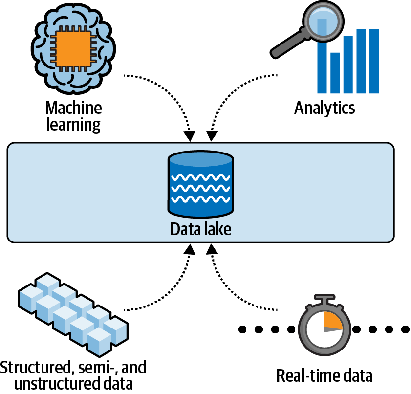
Figure 4-2. A data lake is a centralized and secure repository that enables us to store, govern, discover, and share data at any scale.
Data lakes provide a perfect base for data science and machine learning, as they give us access to large and diverse datasets to train and deploy more accurate models. Building a data lake typically consists of the following (high-level) steps, as shown in Figure 4-3:
-
Set up storage.
-
Move data.
-
Cleanse, prepare, and catalog data.
-
Configure and enforce security and compliance policies.
-
Make data available for analytics.
Each of those steps involves a range of tools and technologies. While we can build a data lake manually from the ground up, there are cloud services available to help us streamline this process, i.e., AWS Lake Formation.
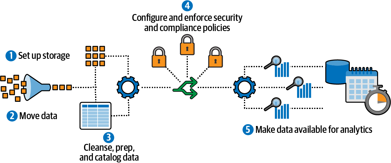
Figure 4-3. Building a data lake involves many steps.
Lake Formation collects and catalogs data from databases and object storage, moves data into an S3-based data lake, secures access to sensitive data, and deduplicates data using machine learning.
Additional capabilities of Lake Formation include row-level security, column-level security, and “governed” tables that support atomic, consistent, isolated, and durable transactions. With row-level and column-level permissions, users only see the data to which they have access. With Lake Formation transactions, users can concurrently and reliably insert, delete, and modify rows across the governed tables. Lake Formation also improves query performance by automatically compacting data storage and optimizing the data layout of governed tables.
S3 has become a popular choice for data lakes, as it offers many ways to ingest our data while enabling cost optimization with intelligent tiering of data, including cold storage and archiving capabilities. S3 also exposes many object-level controls for security and compliance.
On top of the S3 data lake, AWS implements the Lake House Architecture. The Lake House Architecture integrates our S3 data lake with our Amazon Redshift data warehouse for a unified governance model. We will see an example of this architecture in this chapter when we run a query joining data across our Amazon Redshift data warehouse with our S3 data lake.
From a data analysis perspective, another key benefit of storing our data in Amazon S3 is that it shortens the “time to insight” dramatically as we can run ad hoc queries directly on the data in S3. We don’t have to go through complex transformation processes and data pipelines to get our data into traditional enterprise data warehouses, as we will see in the upcoming sections of this chapter.
Import Data into the S3 Data Lake
We are now ready to import our data into S3. We have chosen the Amazon Customer Reviews Dataset as the primary dataset for this book.
The Amazon Customer Reviews Dataset consists of more than 150+ million customer reviews of products across 43 different product categories on the Amazon.com website from 1995 until 2015. It is a great resource for demonstrating machine learning concepts such as natural language processing (NLP), as we demonstrate throughout this book.
Many of us have seen these customer reviews on Amazon.com when contemplating whether to purchase products via the Amazon.com marketplace. Figure 4-4 shows the product reviews section on Amazon.com for an Amazon Echo Dot device.

Figure 4-4. Reviews for an Amazon Echo Dot device. Source: Amazon.com.
Describe the Dataset
Customer reviews are one of Amazon’s most valuable tools for customers looking to make informed purchase decisions. In Amazon’s annual shareholder letters, Jeff Bezos (founder of Amazon) regularly elaborates on the importance of “word of mouth” as a customer acquisition tool. Jeff loves “customers’ constant discontent,” as he calls it:
“We now offer customers…vastly more reviews, content, browsing options, and recommendation features…Word of mouth remains the most powerful customer acquisition tool we have, and we are grateful for the trust our customers have placed in us. Repeat purchases and word of mouth have combined to make Amazon.com the market leader in online bookselling.”
–Jeff Bezos, 1997 Shareholder (“Share Owner”) Letter
Here is the schema for the dataset:
- marketplace
- Two-letter country code (in this case all “US”).
- customer_id
- Random identifier that can be used to aggregate reviews written by a single author.
- review_id
- A unique ID for the review.
- product_id
- The Amazon Standard Identification Number (ASIN).
- product_parent
- The parent of that ASIN. Multiple ASINs (color or format variations of the same product) can roll up into a single product parent.
- product_title
- Title description of the product.
- product_category
- Broad product category that can be used to group reviews.
- star_rating
- The review’s rating of 1 to 5 stars, where 1 is the worst and 5 is the best.
- helpful_votes
- Number of helpful votes for the review.
- total_votes
- Number of total votes the review received.
- vine
- Was the review written as part of the Vine program?
- verified_purchase
- Was the review from a verified purchase?
- review_headline
- The title of the review itself.
- review_body
- The text of the review.
- review_date
- The date the review was written.
The dataset is shared in a public Amazon S3 bucket and is available in two file formats:
-
TSV, a text format: s3://amazon-reviews-pds/tsv
-
Parquet, an optimized columnar binary format: s3://amazon-reviews-pds/parquet
The Parquet dataset is partitioned (divided into subfolders) by the column product_category to further improve query performance. With this, we can use a WHERE clause on product_category in our SQL queries to only read data specific to that category.
We can use the AWS Command Line Interface (AWS CLI) to list the S3 bucket content using the following CLI commands:
-
aws s3 ls s3://amazon-reviews-pds/tsv -
aws s3 ls s3://amazon-reviews-pds/parquet
Note
The AWS CLI tool provides a unified command line interface to Amazon Web Services. We can find more information on how to install and configure the tool.
The following listings show us the available dataset files in TSV format and the Parquet partitioning folder structure.
Dataset files in TSV format:
2017-11-24 13:49:53  648641286 amazon_reviews_us_Apparel_v1_00.tsv.gz
2017-11-24 13:56:36  582145299 amazon_reviews_us_Automotive_v1_00.tsv.gz
2017-11-24 14:04:02  357392893 amazon_reviews_us_Baby_v1_00.tsv.gz
2017-11-24 14:08:11  914070021 amazon_reviews_us_Beauty_v1_00.tsv.gz
2017-11-24 14:17:41 2740337188 amazon_reviews_us_Books_v1_00.tsv.gz
2017-11-24 14:45:50 2692708591 amazon_reviews_us_Books_v1_01.tsv.gz
2017-11-24 15:10:21 1329539135 amazon_reviews_us_Books_v1_02.tsv.gz
...
2017-11-25 08:39:15   94010685 amazon_reviews_us_Software_v1_00.tsv.gz
2017-11-27 10:36:58  872478735 amazon_reviews_us_Sports_v1_00.tsv.gz
2017-11-25 08:52:11  333782939 amazon_reviews_us_Tools_v1_00.tsv.gz
2017-11-25 09:06:08  838451398 amazon_reviews_us_Toys_v1_00.tsv.gz
2017-11-25 09:42:13 1512355451 amazon_reviews_us_Video_DVD_v1_00.tsv.gz
2017-11-25 10:50:22  475199894 amazon_reviews_us_Video_Games_v1_00.tsv.gz
2017-11-25 11:07:59  138929896 amazon_reviews_us_Video_v1_00.tsv.gz
2017-11-25 11:14:07  162973819 amazon_reviews_us_Watches_v1_00.tsv.gz
2017-11-26 15:24:07 1704713674 amazon_reviews_us_Wireless_v1_00.tsv.gz
Dataset files in Parquet format:
PRE product_category=Apparel/
                           PRE product_category=Automotive/
                           PRE product_category=Baby/
                           PRE product_category=Beauty/
                           PRE product_category=Books/
                          ...
                           PRE product_category=Watches/
                           PRE product_category=Wireless/
Note that PRE stands for “prefix.” For now, we can think of prefixes as folders in S3.
It is sometimes useful to use EXPLAIN in our queries to make sure the S3 partitions are being utilized. Spark, for example, will highlight which partitions are being used in Spark SQL. If our query patterns change over time, we may want to revisit updating the existing partitions—or even adding new partitions to match our business needs.
So which data format should we choose? The Parquet columnar file format is definitely preferred when running analytics queries since many analytics queries perform summary statistics (AVG, SUM, STDDEV, etc.) on columns of data. On the other hand, many applications write out data in simple CSV or TSV files, e.g., application log files. So let’s actually assume we don’t have the Parquet files ready to use as this allows us to show us how we can easily get there from CSV or TSV files.
In a first step, let’s copy the TSV data from Amazon’s public S3 bucket into a privately hosted S3 bucket to simulate that process, as shown in Figure 4-5.
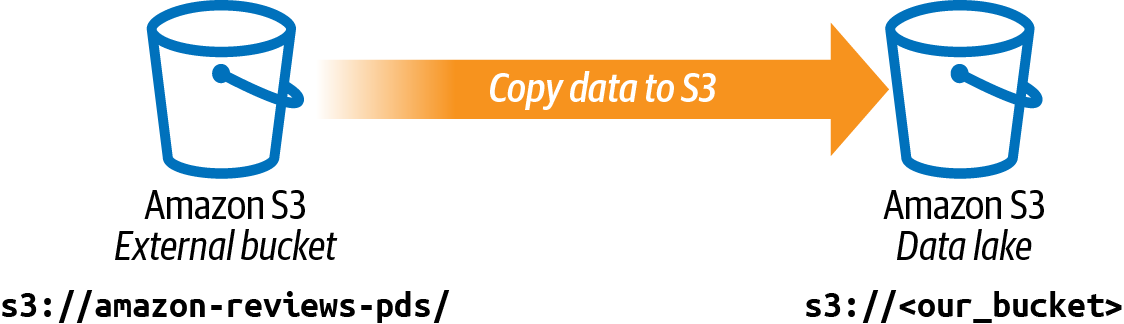
Figure 4-5. We copy the dataset from the public S3 bucket to a private S3 bucket.
We can use the AWS CLI tool again to perform the following steps.
-
Create a new private S3 bucket:
aws s3 mb s3://data-science-on-aws -
Copy the content of the public S3 bucket to our newly created private S3 bucket as follows (only include the files starting with
amazon_reviews_us_, i.e., skipping any index, multilingual, and sample data files in that directory):aws s3 cp --recursive s3://amazon-reviews-pds/tsv/ \ s3://data-science-on-aws/amazon-reviews-pds/tsv/ \ --exclude "*" --include "amazon_reviews_us_*"
We are now ready to use Amazon Athena to register and query the data and transform the TSV files into Parquet.
Query the Amazon S3 Data Lake with Amazon Athena
Amazon Athena is an interactive query service that makes it easy to analyze data in Amazon S3 using standard SQL. With Athena, we can query raw data—including encrypted data—directly from our S3-based data lake. Athena separates compute from storage and lowers the overall time to insight for our business. When we register an Athena table with our S3 data, Athena stores the table-to-S3 mapping. Athena uses the AWS Glue Data Catalog, a Hive Metastore–compatible service, to store the table-to-S3 mapping. We can think of the AWS Glue Data Catalog as a persistent metadata store in our AWS account. Other AWS services, such as Athena and Amazon Redshift Spectrum, can use the data catalog to locate and query data. Apache Spark reads from the AWS Glue Data Catalog, as well.
Besides the data catalog, AWS Glue also provides tools to build ETL (extract-transform-load) workflows. ETL workflows could include the automatic discovery and extraction of data from different sources. We can leverage Glue Studio to visually compose and run ETL workflows without writing code. Glue Studio also provides the single pane of glass to monitor all ETL jobs. AWS Glue executes the workflows on an Apache Spark–based serverless ETL engine.
Athena queries run in parallel inside a dynamically scaled, serverless query engine. Athena will automatically scale the cluster depending on the query and dataset involved. This makes Athena extremely fast on large datasets and frees the user from worrying about infrastructure details.
In addition, Athena supports the Parquet columnar file format with tens of millions of partitions (i.e., by product_category, year, or marketplace) to improve the performance of our queries. For example, if we plan to run frequent queries that group the results by product_category, then we should create a partition in Athena for product_category. Upon creation, Athena will update the AWS Glue Data Catalog accordingly so that future queries will inherit the performance benefits of this new partition.
Athena is based on Presto, an open source, distributed SQL query engine designed for fast, ad hoc data analytics on large datasets. Similar to Apache Spark, Presto uses high-RAM clusters to perform its queries. However, Presto does not require a large amount of disk as it is designed for ad hoc queries (versus automated, repeatable queries) and therefore does not perform the checkpointing required for fault tolerance.
For longer-running Athena jobs, we can listen for query-completion events using Amazon CloudWatch Events. When the query completes, all listeners are notified with the event details, including query success status, total execution time, and total bytes scanned.
With a functionality called Athena Federated Query, we can also run SQL queries across data stored in relational databases, such as Amazon RDS and Aurora, nonrelational databases such as DynamoDB, object storage such as Amazon S3, and custom data sources. This gives us a unified analytics view across data stored in our data warehouse, data lake, and operational databases without the need to actually move the data.
We can access Athena via the AWS Management Console, an API, or an Open Database Connectivity (ODBC) or Java Database Connectivity (JDBC) driver for programmatic access. Let’s take a look at how to use Amazon Athena via the AWS Management Console.
Access Athena from the AWS Console
To use Amazon Athena, we first need to quickly set up the service. First, click on Amazon Athena in the AWS Management Console. If we are asked to set up a “query result” location for Athena in S3, specify an S3 location for the query results (e.g., s3://<BUCKET>/data-science-on-aws/athena/query-results.)
In the next step, we create a database. In the Athena Query Editor, we see a query pane with an example query. We can start typing our query anywhere in the query pane. To create our database, enter the following CREATE DATABASE statement, run the query, and confirm that dsoaws appears in the DATABASE list in the Catalog dashboard:
CREATE DATABASE dsoaws;
When we run CREATE DATABASE and CREATE TABLE queries in Athena with the AWS Glue Data Catalog as our source, we automatically see the database and table metadata entries being created in the AWS Glue Data Catalog.
Register S3 Data as an Athena Table
Now that we have a database, we are ready to create a table based on the Amazon Customer Reviews Dataset. We define the columns that map to the data, specify how the data is delimited, and provide the Amazon S3 path to the data.
Let’s define a “schema-on-read” to avoid the need to predefine a rigid schema when data is written and ingested. In the Athena Console, make sure that dsoaws is selected for DATABASE and then choose New Query. Run the following SQL statement to read the compressed (compression=gzip) files and skip the CSV header (skip.header.line.count=1) at the top of each file. After running the SQL statement, verify that the newly created table, amazon_reviews_tsv, appears on the left under Tables:
CREATE EXTERNAL TABLE IF NOT EXISTS dsoaws.amazon_reviews_tsv(
         marketplace string,
         customer_id string,
         review_id string,
         product_id string,
         product_parent string,
         product_title string,
         product_category string,
         star_rating int,
         helpful_votes int,
         total_votes int,
         vine string,
         verified_purchase string,
         review_headline string,
         review_body string,
         review_date string
) ROW FORMAT DELIMITED FIELDS TERMINATED BY '\t'
LINES TERMINATED BY '\n'
LOCATION 's3://data-science-on-aws/amazon-reviews-pds/tsv'
TBLPROPERTIES ('compressionType'='gzip', 'skip.header.line.count'='1')
Let’s run a sample query like this to check if everything works correctly. This query will produce the results shown in the following table:
SELECT *
FROM dsoaws.amazon_reviews_tsv
WHERE product_category = 'Digital_Video_Download' LIMIT 10
| marketplace | customer_id | review_id | product_id | product_title | product_category |
|---|---|---|---|---|---|
| US | 12190288 | R3FBDHSJD | BOOAYB23D | Enlightened | Digital_Video_Download |
| ... | ... | ... | ... | ... | ... |
Update Athena Tables as New Data Arrives with AWS Glue Crawler
The following code crawls S3 every night at 23:59 UTC and updates the Athena table as new data arrives. If we add another .tar.gz file to S3, for example, we will see the new data in our Athena queries after the crawler completes its scheduled run:
glue = boto3.Session().client(service_name='glue', region_name=region)

create_response = glue.create_crawler(
    Name='amazon_reviews_crawler',
    Role=role,
    DatabaseName='dsoaws',
    Description='Amazon Customer Reviews Dataset Crawler',
    Targets={
        'CatalogTargets': [
            {
                'DatabaseName': 'dsoaws',
                'Tables': [
                    'amazon_reviews_tsv',
                ]
            }
        ]
    },
    Schedule='cron(59 23 * * ? *)', # run every night at 23:59 UTC
     SchemaChangePolicy={
         'DeleteBehavior': 'LOG'
     },
     RecrawlPolicy={
         'RecrawlBehavior': 'CRAWL_EVERYTHING'
     }
)
Create a Parquet-Based Table in Athena
In a next step, we will show how we can easily convert that data into the Apache Parquet columnar file format to improve query performance. Parquet is optimized for columnar-based queries such as counts, sums, averages, and other aggregation-based summary statistics that focus on the column values versus row information.
By storing our data in columnar format, Parquet performs sequential reads for columnar summary statistics. This results in much more efficient data access and “mechanical sympathy” versus having the disk controller jump from row to row and having to reseek to retrieve the column data. If we are doing any type of large-scale data analytics, we should be using a columnar file format like Parquet. We discuss the benefits of Parquet in the performance section.
Note
While we already have the data in Parquet format from the public dataset, we feel that creating a Parquet table is an important-enough topic to demonstrate in this book.
Again, make sure that dsoaws is selected for DATABASE and then choose New Query and run the following CREATE TABLE AS (CTAS) SQL statement:
CREATE TABLE IF NOT EXISTS dsoaws.amazon_reviews_parquet
WITH (format = 'PARQUET', \
        external_location = 's3://<BUCKET>/amazon-reviews-pds/parquet', \
        partitioned_by = ARRAY['product_category']) AS

SELECT marketplace,
         customer_id,
         review_id,
         product_id,
         product_parent,
         product_title,
         star_rating,
         helpful_votes,
         total_votes,
         vine,
         verified_purchase,
         review_headline,
         review_body,
         CAST(YEAR(DATE(review_date)) AS INTEGER) AS year,
         DATE(review_date) AS review_date,
         product_category

FROM dsoaws.amazon_reviews_tsv
As we can see from the query, we’re also adding a new year column to our dataset by converting the review_date string to a date format and then casting the year out of the date. Let’s store the year value as an integer. After running the CTAS query, we should now see the newly created table amazon_reviews_parquet appear as well on the left under Tables. As a last step, we need to load the Parquet partitions. To do so, just issue the following SQL command:
MSCK REPAIR TABLE amazon_reviews_parquet;
Note
We can automate the MSCK REPAIR TABLE command to load the partitions after data ingest from any workflow manager (or use an Lambda function that runs when new data is uploaded to S3).
We can run our sample query again to check if everything works correctly:
SELECT *
FROM dsoaws.amazon_reviews_parquet
WHERE product_category = 'Digital_Video_Download' LIMIT 10
Both tables also have metadata entries in the Hive Metastore–compatible AWS Glue Data Catalog. This metadata defines the schema used by many query and data-processing engines, such as Amazon EMR, Athena, Redshift, Kinesis, SageMaker, and Apache Spark.
In just a few steps, we have set up Amazon Athena to transform the TSV dataset files into the Apache Parquet file format. The query on the Parquet files finished in a fraction of the time compared to the query on the TSV files. We accelerated our query response time by leveraging the columnar Parquet file format and product_category partition scheme.
Continuously Ingest New Data with AWS Glue Crawler
New data is always arriving from applications, and we need a way to register this new data into our system for analytics and model-training purposes. AWS Glue provides sophisticated data-cleansing and machine-learning transformations, including “fuzzy” record deduplication. One way to register the new data from S3 into our AWS Glue Data Catalog is with a Glue Crawler, as shown in Figure 4-6.
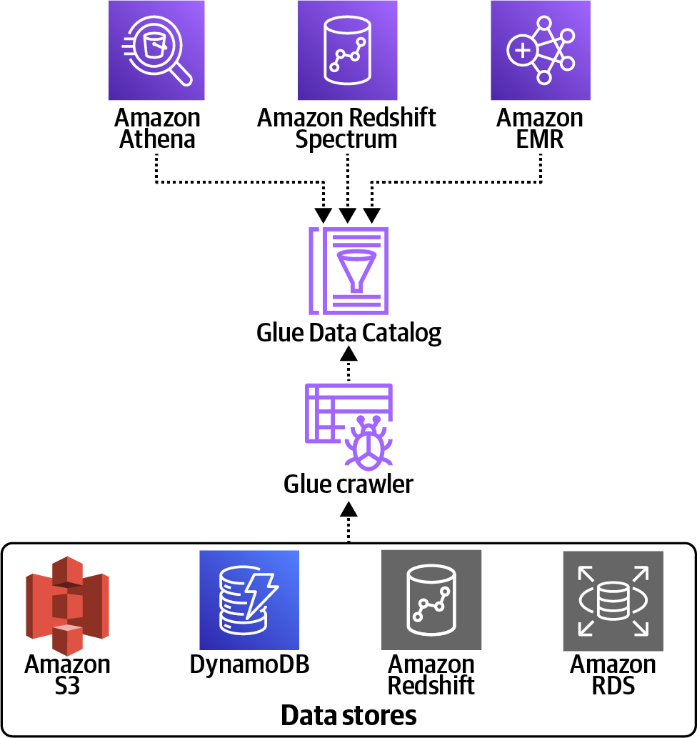
Figure 4-6. Ingest and register data from various data sources with AWS Glue Crawler.
We can trigger the crawler either periodically on a schedule or with, for example, an S3 trigger. The following code creates the crawler and schedules new S3 folders (prefixes) to be ingested every night at 23:59 UTC:
create_response = glue.create_crawler(
    Name='amazon_reviews_crawler',
    Role=role,
    DatabaseName='dsoaws',
    Description='Amazon Customer Reviews Dataset Crawler',
    Targets={
        'CatalogTargets': [
            {
                'DatabaseName': 'dsoaws',
                'Tables': [
                    'amazon_reviews_tsv',
                ]
            }
        ]
    },
    Schedule='cron(59 23 * * ? *)',
     SchemaChangePolicy={
         'DeleteBehavior': 'LOG'
     },
     RecrawlPolicy={
         'RecrawlBehavior': 'CRAWL_NEW_FOLDERS_ONLY'
     }
)
This assumes that we are storing new data in new folders. Typically, we use an S3 prefix that includes the year, month, day, hour, quarter hour, etc. For example, we can store application logs in hourly S3 folders with the following naming convention for the S3 prefix: s3://<S3_BUCKET>/<YEAR>/<MONTH>/<DAY>/<HOUR>/. If we want to crawl all of the data, we can use CRAWL_EVERYTHING for our RecrawlBehavior. We can change the schedule using a different cron() trigger. We can also add a second trigger to start an ETL job to transform and load new data when the scheduled Glue Crawler reaches the SUCCEEDED state.
Build a Lake House with Amazon Redshift Spectrum
One of the fundamental differences between data lakes and data warehouses is that while we ingest and store huge amounts of raw, unprocessed data in our data lake, we normally only load some fraction of our recent data into the data warehouse. Depending on our business and analytics use case, this might be data from the past couple of months, a year, or maybe the past two years. Let’s assume we want to have the past two years of our Amazon Customer Reviews Dataset in a data warehouse to analyze year-over-year customer behavior and review trends. We will use Amazon Redshift as our data warehouse for this.
Amazon Redshift is a fully managed data warehouse that allows us to run complex analytic queries against petabytes of structured data, semistructured, and JSON data. Our queries are distributed and parallelized across multiple nodes. In contrast to relational databases, which are optimized to store data in rows and mostly serve transactional applications, Amazon Redshift implements columnar data storage, which is optimized for analytical applications where we are mostly interested in the data within the individual columns.
Amazon Redshift also includes Amazon Redshift Spectrum, which allows us to directly execute SQL queries from Amazon Redshift against exabytes of unstructured data in our Amazon S3 data lake without the need to physically move the data. Amazon Redshift Spectrum is part of the Lake House Architecture that unifies our S3 data lake and Amazon Redshift data warehouse—including shared security and row-and-column-based access control. Amazon Redshift Spectrum supports various open source storage frameworks, including Apache Hudi and Delta Lake.
Since Amazon Redshift Spectrum automatically scales the compute resources needed based on how much data is being retrieved, queries against Amazon S3 run fast, regardless of the size of our data. Amazon Redshift Spectrum will use pushdown filters, bloom filters, and materialized views to reduce seek time and increase query performance on external data stores like S3. We discuss more performance tips later in “Reduce Cost and Increase Performance”.
Amazon Redshift Spectrum converts traditional ETL into extract-load-transform (ELT) by transforming and cleaning data after it is loaded into Amazon Redshift. We will use Amazon Redshift Spectrum to access our data in S3 and then show how to combine data that is stored in Amazon Redshift with data that is still in S3.
This might sound similar to the approach we showed earlier with Amazon Athena, but note that in this case we show how our business intelligence team can enrich their queries with data that is not stored in the data warehouse itself. Once we have our Redshift cluster set up and configured, we can navigate to the AWS Console and Amazon Redshift and then click on Query Editor to execute commands.
We can leverage our previously created table in Amazon Athena with its metadata and schema information stored in the AWS Glue Data Catalog to access our data in S3 through Amazon Redshift Spectrum. All we need to do is create an external schema in Amazon Redshift, point it to our AWS Glue Data Catalog, and point Amazon Redshift to the database we’ve created.
In the Amazon Redshift Query Editor (or via any other ODBC/JDBC SQL client that we might prefer to use), execute the following command:
CREATE EXTERNAL SCHEMA IF NOT EXISTS athena FROM DATA CATALOG
    DATABASE 'dsoaws'
    IAM_ROLE '<IAM-ROLE>'
    CREATE EXTERNAL DATABASE IF NOT EXISTS
With this command, we are creating a new schema in Amazon Redshift called athena to highlight the data access we set up through our tables in Amazon Athena:
-
FROM DATA CATALOGindicates that the external database is defined in the AWS Glue Data Catalog. -
DATABASErefers to our previously created database in the AWS Glue Data Catalog. -
IAM_ROLEneeds to point to an Amazon Resource Name (ARN) for an IAM role that our cluster uses for authentication and authorization.
IAM is the AWS Identity and Access Management service, which enables us to manage and control access to AWS services and resources in our account. With an IAM role, we can specify the permissions a user or service is granted. In this example, the IAM role must have at a minimum permission to perform a LIST operation on the Amazon S3 bucket to be accessed and a GET operation on the Amazon S3 objects the bucket contains. If the external database is defined in an Amazon Athena data catalog, the IAM role must have permission to access Athena unless CATALOG_ROLE is specified. We will go into more details on IAM in a later section of this chapter when we discuss how we can secure our data.
If we now select athena in the Schema dropdown menu in the Amazon Redshift Query Editor, we can see that our two tables, amazon_reviews_tsv and amazon_reviews_parquet, appear, which we created with Amazon Athena. Let’s run a sample query again to make sure everything works. In the Query Editor, run the following command:
SELECT
    product_category,
    COUNT(star_rating) AS count_star_rating
FROM
    athena.amazon_reviews_tsv
GROUP BY
    product_category
ORDER BY
    count_star_rating DESC
We should see results similar to the following table:
| product_category | count_star_rating |
|---|---|
| Books | 19531329 |
| Digital_Ebook_Purchase | 17622415 |
| Wireless | 9002021 |
| ... | ... |
So with just one command, we now have access and can query our S3 data lake from Amazon Redshift without moving any data into our data warehouse. This is the power of Amazon Redshift Spectrum.
But now, let’s actually copy some data from S3 into Amazon Redshift. Let’s pull in customer reviews data from the year 2015.
First, we create another Amazon Redshift schema called redshift with the following SQL command:
CREATE SCHEMA IF NOT EXISTS redshift
Next, we will create a new table that represents our customer reviews data. We will also add a new column and add year to our table:
        CREATE TABLE IF NOT EXISTS redshift.amazon_reviews_tsv_2015(
             marketplace varchar(2) ENCODE zstd,
             customer_id varchar(8) ENCODE zstd,
             review_id varchar(14) ENCODE zstd,
             product_id varchar(10) ENCODE zstd DISTKEY,
             product_parent varchar(10) ENCODE zstd,
             product_title varchar(400) ENCODE zstd,
             product_category varchar(24) ENCODE raw,
             star_rating int ENCODE az64,
             helpful_votes int ENCODE zstd,
             total_votes int ENCODE zstd,
             vine varchar(1) ENCODE zstd,
             verified_purchase varchar(1) ENCODE zstd,
             review_headline varchar(128) ENCODE zstd,
             review_body varchar(65535) ENCODE zstd,
             review_date varchar(10) ENCODE bytedict,
             year int ENCODE az64)  SORTKEY (product_category)
In the performance section, we will dive deep into the SORTKEY, DISTKEY, and ENCODE attributes. For now, let’s copy the data from S3 into our new Amazon Redshift table and run some sample queries.
For such bulk inserts, we can either use a COPY command or an INSERT INTO command. In general, the COPY command is preferred, as it loads data in parallel and more efficiently from Amazon S3, or other supported data sources.
If we are loading data or a subset of data from one table into another, we can use the INSERT INTO command with a SELECT clause for high-performance data insertion. As we’re loading our data from the athena.amazon_reviews_tsv table, let’s choose this option:
INSERT
INTO
    redshift.amazon_reviews_tsv_2015
    SELECT
        marketplace,
        customer_id,
        review_id,
        product_id,
        product_parent,
        product_title,
        product_category,
        star_rating,
        helpful_votes,
        total_votes,
        vine,
        verified_purchase,
        review_headline,
        review_body,
        review_date,
        CAST(DATE_PART_YEAR(TO_DATE(review_date,
        'YYYY-MM-DD')) AS INTEGER) AS year
    FROM
        athena.amazon_reviews_tsv
    WHERE
        year = 2015
We use a date conversion to parse the year out of our review_date column and store it in a separate year column, which we then use to filter records from 2015. This is an example of how we can simplify ETL tasks, as we put our data transformation logic directly in a SELECT query and ingest the result into Amazon Redshift.
Another way to optimize our tables would be to create them as a sequence of time-series tables, especially when our data has a fixed retention period. Let’s say we want to store data of the last two years (24 months) in our data warehouse and update with new data once a month.
If we create one table per month, we can easily remove old data by running a DROP TABLE command on the corresponding table. This approach is much faster than running a large-scale DELETE process and also saves us from having to run a subsequent VACUUM process to reclaim space and resort the rows.
To combine query results across tables, we can use a UNION ALL view. Similarly, when we need to delete old data, we remove the dropped table from the UNION ALL view.
Here is an example of a UNION ALL view across two tables with customer reviews from years 2014 and 2015—assuming we have one table each for 2014 and 2015 data. The following table shows the results of the query:
SELECT
    product_category,
    COUNT(star_rating) AS count_star_rating,
    year
FROM
    redshift.amazon_reviews_tsv_2014
GROUP BY
    redshift.amazon_reviews_tsv_2014.product_category,
    year
UNION
ALL SELECT
    product_category,
    COUNT(star_rating) AS count_star_rating,
    year
FROM
    redshift.amazon_reviews_tsv_2015
GROUP BY
    redshift.amazon_reviews_tsv_2015.product_category,
    year
ORDER BY
    count_star_rating DESC,
    year ASC
| product_category | count_star_rating | year |
|---|---|---|
| Digital_Ebook_Purchase | 6615914 | 2014 |
| Digital_Ebook_Purchase | 4533519 | 2015 |
| Books | 3472631 | 2014 |
| Wireless | 2998518 | 2015 |
| Wireless | 2830482 | 2014 |
| Books | 2808751 | 2015 |
| Apparel | 2369754 | 2015 |
| Home | 2172297 | 2015 |
| Apparel | 2122455 | 2014 |
| Home | 1999452 | 2014 |
Now, let’s actually run a query and combine data from Amazon Redshift with data that is still in S3. Let’s take the data from the previous query for the years 2015 and 2014 and query Athena/S3 for the years 2013–1995 by running this command:
SELECT
    year,
    product_category,
    COUNT(star_rating) AS count_star_rating
FROM
    redshift.amazon_reviews_tsv_2015
GROUP BY
    redshift.amazon_reviews_tsv_2015.product_category,
    year
UNION
ALL SELECT
    year,
    product_category,
    COUNT(star_rating) AS count_star_rating
FROM
    redshift.amazon_reviews_tsv_2014
GROUP BY
    redshift.amazon_reviews_tsv_2014.product_category,
    year
UNION
ALL SELECT
    CAST(DATE_PART_YEAR(TO_DATE(review_date,
    'YYYY-MM-DD')) AS INTEGER) AS year,
    product_category,
    COUNT(star_rating) AS count_star_rating
FROM
    athena.amazon_reviews_tsv
WHERE
    year <= 2013
GROUP BY
    athena.amazon_reviews_tsv.product_category,
    year
ORDER BY
    product_category ASC,
    year DESC
| year | product_category | count_star_rating |
|---|---|---|
| 2015 | Apparel | 4739508 |
| 2014 | Apparel | 4244910 |
| 2013 | Apparel | 854813 |
| 2012 | Apparel | 273694 |
| 2011 | Apparel | 109323 |
| 2010 | Apparel | 57332 |
| 2009 | Apparel | 42967 |
| 2008 | Apparel | 33761 |
| 2007 | Apparel | 25986 |
| 2006 | Apparel | 7293 |
| 2005 | Apparel | 3533 |
| 2004 | Apparel | 2357 |
| 2003 | Apparel | 2147 |
| 2002 | Apparel | 907 |
| 2001 | Apparel | 5 |
| 2000 | Apparel | 6 |
| 2015 | Automotive | 2609750 |
| 2014 | Automotive | 2350246 |
Export Amazon Redshift Data to S3 Data Lake as Parquet
Amazon Redshift Data Lake Export gives us the ability to unload the result of an Amazon Redshift query to our S3 data lake in the optimized Apache Parquet columnar file format. This enables us to share any data transformation and enrichment we have done in Amazon Redshift back into our S3 data lake in an open format. Unloaded data is automatically registered in the AWS Glue Data Catalog to be used by any Hive Metastore–compatible query engines, including Amazon Athena, EMR, Kinesis, SageMaker, and Apache Spark.
We can specify one or more partition columns so that unloaded data is automatically partitioned into folders in our Amazon S3 bucket. For example, we can choose to unload our customer reviews data and partition it by product_category.
We can simply run the following SQL command to unload our 2015 customer reviews data in Parquet file format into S3, partitioned by product_category:
UNLOAD (
   'SELECT marketplace, customer_id, review_id, product_id, product_parent,
     product_title, product_category, star_rating, helpful_votes, total_votes,
     vine, verified_purchase, review_headline, review_body, review_date, year
     FROM redshift.amazon_reviews_tsv_2015')
TO 's3://data-science-on-aws/amazon-reviews-pds/parquet-from-redshift/2015'
IAM_ROLE '<IAM_ROLE>'
PARQUET PARALLEL ON
PARTITION BY (product_category)
We can use the AWS CLI tool again to list the S3 folder and see our unloaded data from 2015 in Parquet format:
aws s3 ls s3://data-science-on-aws/amazon-reviews-pds/parquet-from-redshift/2015
Choose Between Amazon Athena and Amazon Redshift
Amazon Athena is the preferred choice when running ad hoc SQL queries on data that is stored in Amazon S3. It doesn’t require us to set up or manage any infrastructure resources—we don’t need to move any data. It supports structured, unstructured, and semistructured data. With Athena, we are defining a “schema on read”—we basically just log in, create a table, and start running queries.
Amazon Redshift is targeted for modern data analytics on petabytes of structured data. Here, we need to have a predefined “schema on write.” Unlike serverless Athena, Amazon Redshift requires us to create a cluster (compute and storage resources), ingest the data, and build tables before we can start to query but caters to performance and scale. So for highly relational data with a transactional nature (data gets updated), workloads that involve complex joins, or subsecond latency requirements, Amazon Redshift is the right choice.
Athena and Amazon Redshift are optimized for read-heavy analytics workloads; they are not replacements for write-heavy, relational databases such as Amazon Relational Database Service (RDS) and Aurora. At a high level, use Athena for exploratory analytics and operational debugging; use Amazon Redshift for business-critical reports and dashboards.
Reduce Cost and Increase Performance
In this section, we want to provide some tips and tricks to reduce cost and increase performance during data ingestion, including file formats, partitions, compression, and sort/distribution keys. We will also demonstrate how to use Amazon S3 Intelligent-Tiering to lower our storage bill.
S3 Intelligent-Tiering
We introduced Amazon S3 in this chapter as a scalable, durable storage service for building shared datasets, such as data lakes in the cloud. And while we keep the S3 usage fairly simple in this book, the service actually offers us a variety of options to optimize our storage cost as our data grows.
Depending on our data’s access frequency patterns and service-level agreement (SLA) needs, we can choose from various Amazon S3 storage classes. Table 4-1 compares the Amazon S3 storage classes in terms of data access frequency and data retrieval time.
| From frequent access | To infrequent access | ||||
|---|---|---|---|---|---|
| S3 Standard (default storage class) | S3 Intelligent-Tiering | S3 Standard-IA | S3 One Zone-IA | Amazon S3 Glacier | Amazon S3 Glacier Deep Archive |
| General-purpose storage Active, frequently accessed data Access in milliseconds |
Data with unknown or changing access patterns Access in milliseconds Opt in for automatic archiving |
Infrequently accessed (IA) data Access in milliseconds |
Lower durability (one Zvailability zone) Re-creatable data Access in milliseconds |
Archive data Access in minutes or hours |
Long-term archive data Access in hours |
But how do we know which objects to move? Imagine our S3 data lake has grown over time and we possibly have billions of objects across several S3 buckets in the S3 Standard storage class. Some of those objects are extremely important, while we haven’t accessed others maybe in months or even years. This is where S3 Intelligent-Tiering comes into play.
Amazon S3 Intelligent-Tiering automatically optimizes our storage cost for data with changing access patterns by moving objects between the frequent-access tier optimized for frequent use of data and the lower-cost infrequent-access tier optimized for less-accessed data. Intelligent-Tiering monitors our access patterns and auto-tiers on a granular object level without performance impact or any operational overhead.
Parquet Partitions and Compression
Athena supports the Parquet columnar format for large-scale analytics workloads. Parquet enables the following performance optimizations for our queries:
- Partitions and pushdowns
- Partitions are physical groupings of data on disk to match our query patterns (i.e.,
SELECT * FROM reviews WHERE product_category='Books'). Modern query engines like Athena, Amazon Redshift, and Apache Spark will “pushdown” theWHEREinto the physical storage system to allow the disk controller to seek once and read all relevant data in one scan without randomly skipping to different areas of the disk. This improves query performance even with solid state drives (SSDs), which have a lower seek time than traditional, media-based disks. - Dictionary encoding/compression
- When a small number of categorical values are stored together on disk (i.e.,
product_category, which has 43 total values in our dataset), the values can be compressed into a small number of bits to represent each value (i.e.,Books,Lawn_and_Garden,Software, etc.) versus storing the entire string. - Type compression
- When values of a similar type (i.e., String, Date, Integer) are stored together on disk, the values can be compressed together: (String, String), (Date, Date), (Integer, Integer). This compression is more efficient than if the values were stored separately on disk in a row-wise manner: (String, Date, Integer), (String, Date, Integer)
- Vectorized aggregations
- Because column values are stored together on disk, the disk controller needs to only perform one disk seek to find the beginning of the data. From that point, it will scan the data to perform the aggregation. Additionally, modern chips/processors offer high-performance vectorization instructions to perform calculations on large amounts of data versus flushing data in and out of the various data caches (L1, L2) or main memory.
See an example of row versus columnar data format in Figure 4-7.
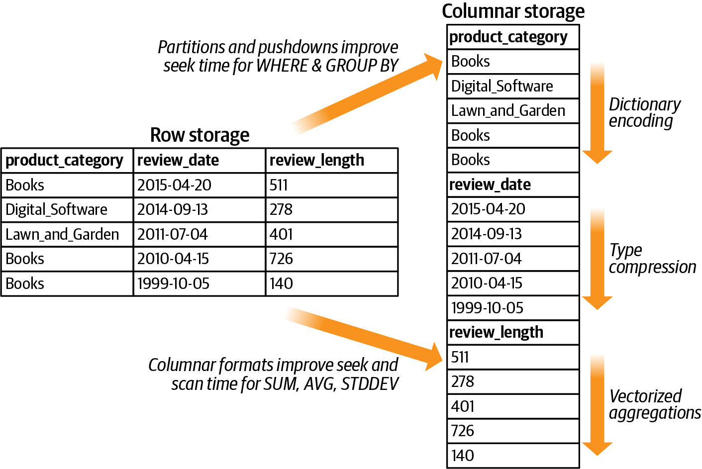
Figure 4-7. Using a columnar data format such as Parquet, we can apply various performance optimizations for query execution and data encoding.
Amazon Redshift Table Design and Compression
Here is the CREATE TABLE statement that we used to create the Amazon Redshift tables:
CREATE TABLE IF NOT EXISTS redshift.amazon_reviews_tsv_2015(
             marketplace varchar(2) ENCODE zstd,
             customer_id varchar(8) ENCODE zstd,
             review_id varchar(14) ENCODE zstd,
             product_id varchar(10) ENCODE zstd DISTKEY,
             product_parent varchar(9) ENCODE zstd,
             product_title varchar(400) ENCODE zstd,
             product_category varchar(24) ENCODE raw,
             star_rating int ENCODE az64,
             helpful_votes int ENCODE zstd,
             total_votes int ENCODE zstd,
             vine varchar(1) ENCODE zstd,
             verified_purchase varchar(1) ENCODE zstd,
             review_headline varchar(128) ENCODE zstd,
             review_body varchar(65535) ENCODE zstd,
             review_date varchar(10) ENCODE bytedict,
             year int ENCODE az64)  SORTKEY (product_category)
When we create a table, we can specify one or more columns as the SORTKEY. Amazon Redshift stores the data on disk in sorted order according to the SORTKEY. Hence, we can optimize our table by choosing a SORTKEY that reflects our most frequently used query types. If we query a lot of recent data, we can specify a timestamp column as the SORTKEY. If we frequently query based on range or equality filtering on one column, we should choose that column as the SORTKEY. As we are going to run a lot of queries in the next chapter filtering on product_category, let’s choose that one as our SORTKEY.
Tip
Amazon Redshift Advisor continuously recommends SORTKEYs for frequently queried tables. Advisor will generate an ALTER TABLE command that we run without having to re-create the tables—without impacting concurrent read and write queries. Note that Advisor does not provide recommendations if it doesn’t see enough data (queries) or if the benefits are relatively small.
We can also define a distribution style for every table. When we load data into a table, Amazon Redshift distributes the rows of the table among our cluster nodes according to the table’s distribution style. When we perform a query, the query optimizer redistributes the rows to the cluster nodes as needed to perform any joins and aggregations. So our goal should be to optimize the rows distribution to minimize data movements. There are three distribution styles from which we can choose:
KEYdistribution- Distribute the rows according to the values in one column.
ALLdistribution- Distribute a copy of the entire table to every node.
EVENdistribution- The rows are distributed across all nodes in a round-robin fashion, which is the default distribution style.
For our table, we’ve chosen KEY distribution based on product_id, as this column has a high cardinality, shows an even distribution, and can be used to join with other tables.
At any time, we can use EXPLAIN on our Amazon Redshift queries to make sure the DISTKEY and SORTKEY are being utilized. If our query patterns change over time, we may want to revisit changing these keys.
In addition, we are using compression for most columns to reduce the overall storage footprint and reduce our cost. Table 4-2 analyzes the compression used for each Amazon Redshift column in our schema.
| Column | Data type | Encoding | Explanation |
|---|---|---|---|
| marketplace | varchar(2) | zstd | Low cardinality, too small for higher compression overhead |
| customer_id | varchar(8) | zstd | High cardinality, relatively few repeat values |
| review_id | varchar(14) | zstd | Unique, unbounded cardinality, no repeat values |
| product_id | varchar(10) | zstd | Unbounded cardinality, relatively low number of repeat values |
| product_parent | varchar(10) | zstd | Unbounded cardinality, relatively low number of repeat words |
| product_title | varchar(400) | zstd | Unbounded cardinality, relatively low number of repeat words |
| product_category | varchar(24) | raw | Low cardinality, many repeat values, but first SORT key is raw |
| star_rating | int | az64 | Low cardinality, many repeat values |
| helpful_votes | int | zstd | Relatively high cardinality |
| total_votes | int | zstd | Relatively high cardinality |
| vine | varchar(1) | zstd | Low cardinality, too small to incur higher compression overhead |
| verified_purchase | varchar(1) | zstd | Low cardinality, too small to incur higher compression overhead |
| review_headline | varchar(128) | zstd | Varying length text, high cardinality, low repeat words |
| review_body | varchar(65535) | zstd | Varying length text, high cardinality, low repeat words |
| review_date | varchar(10) | bytedict | Fixed length, relatively low cardinality, many repeat values |
| year | int | az64 | Low cardinality, many repeat values |
Note
While AWS CEO Andy Jassy maintains “there is no compression algorithm for experience,” there is a compression algorithm for data. Compression is a powerful tool for the ever-growing world of big data. All modern big data processing tools are compression-friendly, including Amazon Athena, Redshift, Parquet, pandas, and Apache Spark. Using compression on small values such as varchar(1) may not improve performance. However, due to native hardware support, there are almost no drawbacks to using compression.
zstd is a generic compression algorithm that works across many different data types and column sizes. The star_rating and year fields are set to the default az64 encoding applied to most numeric and date fields. For most columns, we gain a quick win by using the default az64 encoding for integers and overriding the default lzo encoding in favor of the flexible zstd encoding for everything else, including text.
We are using bytedict for review_date to perform dictionary encoding on the string-based dates (YYYY-MM-DD). While it seemingly has a large number of unique values, review_date actually contains a small number of unique values because there are only ~7,300 (365 days per year × 20 years) days in a 20-year span. This cardinality is low enough to capture all of the possible dates in just a few bits versus using a full varchar(10) for each date.
While product_category is a great candidate for bytedict dictionary encoding, it is our first (and only, in this case) SORTKEY. As a performance best practice, the first SORTKEY should not be compressed.
While marketplace, product_category, vine, and verified_purchase seem to be good candidates for bytedict, they are too small to benefit from the extra overhead. For now, we leave them as zstd.
If we have an existing Amazon Redshift table to optimize, we can run the ANALYZE COMPRESSION command in Amazon Redshift to generate a report of suggested compression encodings as follows:
ANALYZE COMPRESSION redshift.customer_reviews_tsv_2015
The result will be a table like the following showing the % improvement in compression if we switch to another encoding:
| Column | Encoding | Estimated reduction (%) |
|---|---|---|
marketplace |
zstd |
90.84 |
customer_id |
zstd |
38.88 |
review_id |
zstd |
36.56 |
product_id |
zstd |
44.15 |
product_parent |
zstd |
44.03 |
product_title |
zstd |
30.72 |
product_category |
zstd |
99.95 |
star_rating |
az64 |
0 |
helpful_votes |
zstd |
47.58 |
total_votes |
zstd |
39.75 |
vine |
zstd |
85.03 |
verified_purchase |
zstd |
73.09 |
review_headline |
zstd |
30.55 |
review_body |
zstd |
32.19 |
review_date |
bytedict |
64.1 |
year |
az64 |
0 |
We performed this analysis on a version of the CREATE TABLE that did not specify any ENCODE attributes. By default, Amazon Redshift will use az64 for numerics/dates and lzo for everything else (hence the 0% gain for the az64 suggestions). We can also use the ALTER TABLE statement to change the compression used for each column.
Keep in mind that these are just suggestions and not always appropriate for our specific environment. We should try different encodings for our dataset and query the STV_BLOCKLIST table to compare the % reduction in physical number of blocks. For example, the analyzer recommends using zstd for our SORTKEY, product_category, but our experience shows that query performance suffers when we compress the SORTKEY. We are using the extra disk space to improve our query performance.
Amazon Redshift supports automatic table optimization and other self-tuning capabilities that leverage machine learning to optimize peak performance and adapt to shifting workloads. The performance optimizations include automatic vacuum deletes, intelligent workload management, automatic table sorts, and automatic selection of distribution and sort keys.
Use Bloom Filters to Improve Query Performance
Amazon Redshift is a distributed query engine and S3 is a distributed object store. Distributed systems consist of many cluster instances. To improve performance of distributed queries, we need to minimize the number of instances that are scanned and the amount of data transferred between the instances.
Bloom filters, probabilistic and memory-efficient data structures, help answer the question, “Does this specific cluster instance contain data that might be included in the query results?” Bloom filters answer with either a definite NO or a MAYBE. If the bloom filter answered with a NO, the engine will completely skip that cluster instance and scan the remaining instances where the bloom filter answered with a MAYBE.
By filtering out rows of data that do not match the given query, bloom filters result in huge performance gains for join queries. And since bloom filtering happens close to the data source, data transfer is minimized between the nodes in the distributed cluster during join queries. This ultimately increases query performance for data stores such as S3.
Amazon Redshift Spectrum actually automatically creates and manages bloom filters on external data such as S3, but we should be aware of their importance in improving query performance on distributed data stores. Bloom filters are a pattern used throughout all of distributed computing, including distributed query engines.
Materialized Views in Amazon Redshift Spectrum
Materialized views provide repeatable and predictable query performance on external data sources such as S3. They pretransform and prejoin data before SQL queries are executed. Materialized views can be updated either manually or on a predefined schedule using Amazon Redshift Spectrum.
Summary
In this chapter, we provided an overview on how we can load our data into Amazon S3, discussed the value of an S3 data lake, and showed how we can leverage services like Amazon Athena to run ad hoc SQL queries across the data in S3 without the need to physically move the data. We showed how to continuously ingest new application data using AWS Glue Crawler. We also introduced our dataset, the Amazon Customer Reviews Dataset, which we will be using through the rest of this book.
As different use cases require data in different formats, we elaborated on how we can use Athena to convert tab-separated data into query-optimized, columnar Parquet data.
Data in our S3 data lake often needs to be accessed not only by the data science and machine learning teams but also by business intelligence teams. We introduced the Lake House Architecture based on Amazon Redshift, AWS’s petabyte-scale cloud data warehouse. We showed how to use Amazon Redshift Spectrum to combine queries across data stores, including Amazon Redshift and S3.
To conclude this chapter, we discussed the various data compression formats and S3 tiering options, showing how they can reduce cost and improve query performance.
In Chapter 5 we will explore the dataset in more detail. We will run queries to understand and visualize our datasets. We will also show how to detect data anomalies with Apache Spark and Amazon SageMaker Processing Jobs.
Get Data Science on AWS now with the O’Reilly learning platform.
O’Reilly members experience books, live events, courses curated by job role, and more from O’Reilly and nearly 200 top publishers.

