Python for Excel

Chapter 4. NumPy Foundations

As you may recall from Chapter 1, NumPy is the core package for scientific computing in Python, providing support for array-based calculations and linear algebra. As NumPy is the backbone of pandas, I am going to introduce its basics in this chapter: after explaining what a NumPy array is, we will look into vectorization and broadcasting, two important concepts that allow you to write concise mathematical code and that you will find again in pandas. After that, we’re going to see why NumPy offers special functions called universal functions before we wrap this chapter up by learning how to get and set values of an array and by explaining the difference between a view and a copy of a NumPy array. Even if we will hardly use NumPy directly in this book, knowing its basics will make it easier to learn pandas in the next chapter.

Getting Started with NumPy

In this section, we’ll learn about one- and two-dimensional NumPy arrays and what’s behind the technical terms vectorization, broadcasting, and universal function.

NumPy Array

To perform array-based calculations with nested lists, as we met them in the last chapter, you would have to write some sort of loop. For example, to add a number to every element in a nested list, you can use the following nested list comprehension:

In [1]: matrix = [[1, 2, 3],
                  [4, 5, 6],
                  [7, 8, 9]]

In [2]: [[i + 1 for i in row] for row in matrix]

Out[2]: [[2, 3, 4], [5, 6, 7], [8, 9, 10]]

This isn’t very readable and more importantly, if you do this with big arrays, looping through each element becomes very slow. Depending on your use case and the size of the arrays, calculating with NumPy arrays instead of Python lists can make your calculations from a couple of times to around a hundred times faster. NumPy achieves this performance by making use of code that was written in C or Fortran—these are compiled programming languages that are much faster than Python. A NumPy array is an N-dimensional array for homogenous data. Homogenous means that all elements in the array need to be of the same data type. Most commonly, you are dealing with one- and two-dimensional arrays of floats as schematically displayed in Figure 4-1.

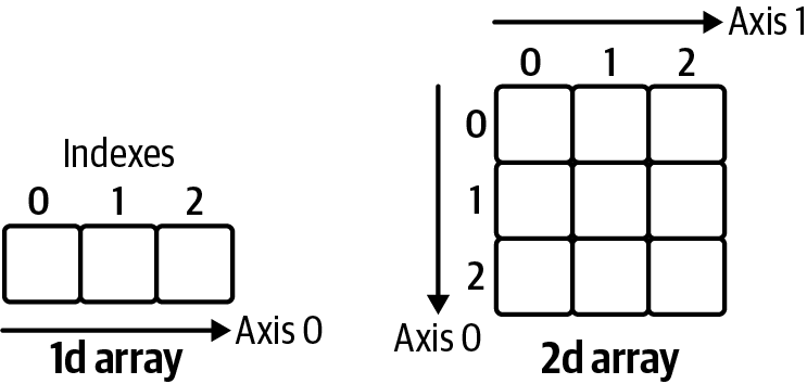
Figure 4-1. A one-dimensional and two-dimensional NumPy array

Let’s create a one- and two-dimensional array to work with throughout this chapter:

In [3]: # First, let's import NumPy
        import numpy as np

In [4]: # Constructing an array with a simple list results in a 1d array
        array1 = np.array([10, 100, 1000.])

In [5]: # Constructing an array with a nested list results in a 2d array
        array2 = np.array([[1., 2., 3.],
                           [4., 5., 6.]])

Array Dimension

It’s important to note the difference between a one- and two-dimensional array: a one-dimensional array has only one axis and hence does not have an explicit column or row orientation. While this behaves like arrays in VBA, you may have to get used to it if you come from a language like MATLAB, where one-dimensional arrays always have a column or row orientation.

Even if array1 consists of integers except for the last element (which is a float), the homogeneity of NumPy arrays forces the data type of the array to be float64, which is capable of accommodating all elements. To learn about an array’s data type, access its dtype attribute:

In [6]: array1.dtype

Out[6]: dtype('float64')

Since dtype gives you back float64 instead of float which we met in the last chapter, you may have guessed that NumPy uses its own numerical data types, which are more granular than Python’s data types. This usually isn’t an issue though, as most of the time, conversion between the different data types in Python and NumPy happens automatically. If you ever need to explicitly convert a NumPy data type to one of Python’s basic data types, simply use the corresponding constructor (I will say more about accessing an element from an array shortly):

In [7]: float(array1[0])

Out[7]: 10.0

For a full list of NumPy’s data types, see the NumPy docs. With NumPy arrays, you can write simple code to perform array-based calculations, as we will see next.

Vectorization and Broadcasting

If you build the sum of a scalar and a NumPy array, NumPy will perform an element-wise operation, which means that you don’t have to loop through the elements yourself. The NumPy community refers to this as vectorization. It allows you to write concise code, practically representing the mathematical notation:

In [8]: array2 + 1

Out[8]: array([[2., 3., 4.],
               [5., 6., 7.]])

Scalar

Scalar refers to a basic Python data type like a float or a string. This is to differentiate them from data structures with multiple elements like lists and dictionaries or one- and two-dimensional NumPy arrays.

The same principle applies when you work with two arrays: NumPy performs the operation element-wise:

In [9]: array2 * array2

Out[9]: array([[ 1.,  4.,  9.],
               [16., 25., 36.]])

If you use two arrays with different shapes in an arithmetic operation, NumPy extends—if possible—the smaller array automatically across the larger array so that their shapes become compatible. This is called broadcasting:

In [10]: array2 * array1

Out[10]: array([[  10.,  200., 3000.],
                [  40.,  500., 6000.]])

To perform matrix multiplications or dot products, use the @ operator:¹

In [11]: array2 @ array2.T  # array2.T is a shortcut for array2.transpose()

Out[11]: array([[14., 32.],
                [32., 77.]])

Don’t be intimidated by the terminology I’ve introduced in this section such as scalar, vectorization, or broadcasting! If you have ever worked with arrays in Excel, this should all feel very natural as shown in Figure 4-2. The screenshot is taken from array_calculations.xlsx, which you will find in the xl directory of the companion repository.

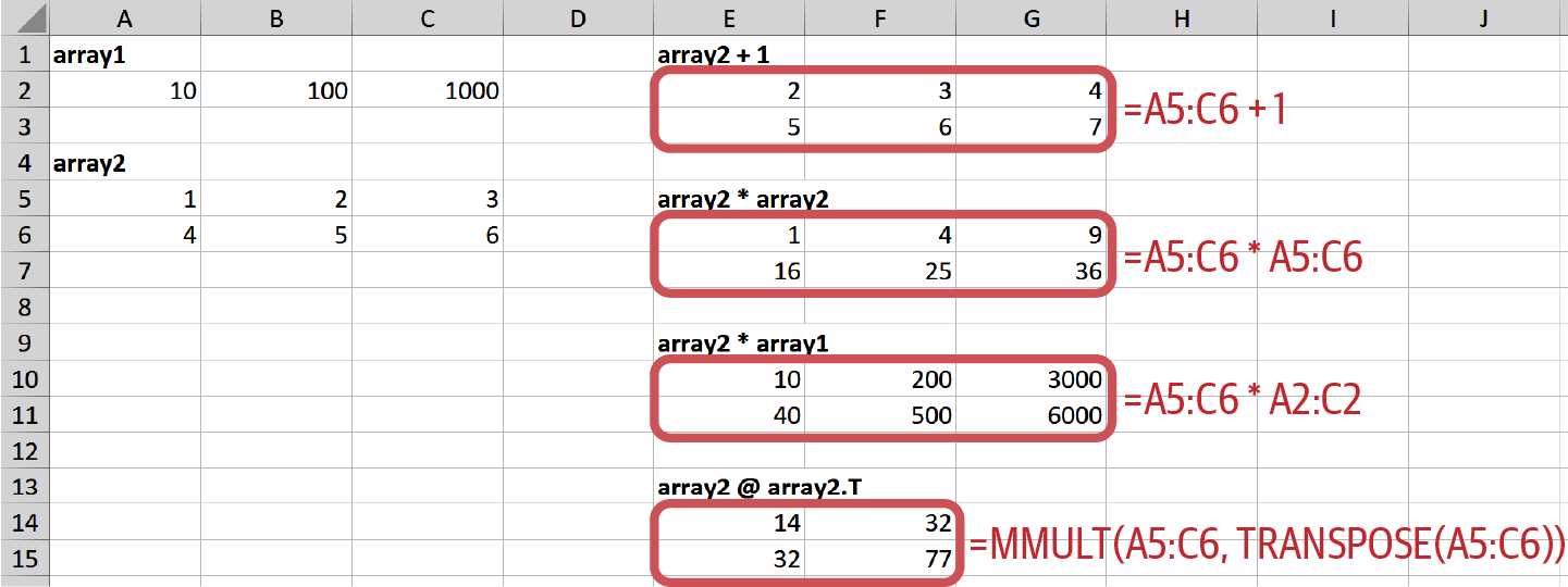
Figure 4-2. Array-based calculations in Excel

You know now that arrays perform arithmetic operations element-wise, but how can you apply a function on every element in an array? This is what universal functions are here for.

Universal Functions (ufunc)

Universal functions (ufunc) work on every element in a NumPy array. For example, if you use Python’s standard square root function from the math module on a NumPy array, you will get an error:

In [12]: import math

In [13]: math.sqrt(array2)  # This will raise en Error

---------------------------------------------------------------------------
TypeError                                 Traceback (most recent call last)
<ipython-input-13-5c37e8f41094> in <module>
----> 1 math.sqrt(array2)  # This will raise en Error

TypeError: only size-1 arrays can be converted to Python scalars

You could, of course, write a nested loop to get the square root of every element, then build a NumPy array again from the result:

In [14]: np.array([[math.sqrt(i) for i in row] for row in array2])

Out[14]: array([[1.        , 1.41421356, 1.73205081],
                [2.        , 2.23606798, 2.44948974]])

This will work in cases where NumPy doesn’t offer a ufunc and the array is small enough. However, if NumPy has a ufunc, use it, as it will be much faster with big arrays—apart from being easier to type and read:

In [15]: np.sqrt(array2)

Out[15]: array([[1.        , 1.41421356, 1.73205081],
                [2.        , 2.23606798, 2.44948974]])

Some of NumPy’s ufuncs, like sum, are additionally available as array methods: if you want the sum of each column, do the following:

In [16]: array2.sum(axis=0)  # Returns a 1d array

Out[16]: array([5., 7., 9.])

The argument axis=0 refers to the axis along the rows while axis=1 refers to the axis along the columns, as depicted in Figure 4-1. Leaving the axis argument away sums up the whole array:

In [17]: array2.sum()

Out[17]: 21.0

You will meet more NumPy ufuncs throughout this book, as they can be used with pandas DataFrames.

So far, we’ve always worked with the entire array. The next section shows you how to manipulate parts of an array and introduces a few helpful array constructors.

Creating and Manipulating Arrays

I’ll start this section by getting and setting specific elements of an array before introducing a few useful array constructors, including one to create pseudorandom numbers that you could use for a Monte Carlo simulation. I’ll wrap this section up by explaining the difference between a view and a copy of an array.

Getting and Setting Array Elements

In the last chapter, I showed you how to index and slice lists to get access to specific elements. When you work with nested lists like matrix from the first example in this chapter, you can use chained indexing: matrix[0][0] will get you the first element of the first row. With NumPy arrays, however, you provide the index and slice arguments for both dimensions in a single pair of square brackets:

numpy_array[row_selection, column_selection]

For one-dimensional arrays, this simplifies to numpy_array[selection]. When you select a single element, you will get back a scalar; otherwise, you will get back a one- or two-dimensional array. Remember that slice notation uses a start index (included) and an end index (excluded) with a colon in between, as in start:end. By leaving away the start and end index, you are left with a colon, which therefore stands for all rows or all columns in a two-dimensional array. I have visualized a few examples in Figure 4-3, but you may also want to give Figure 4-1 another look, as the indices and axes are labeled there. Remember, by slicing a column or row of a two-dimensional array, you end up with a one-dimensional array, not with a two-dimensional column or row vector!

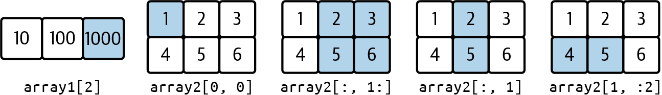
Figure 4-3. Selecting elements of a NumPy array

Play around with the examples shown in Figure 4-3 by running the following code:

In [18]: array1[2]  # Returns a scalar

Out[18]: 1000.0

In [19]: array2[0, 0]  # Returns a scalar

Out[19]: 1.0

In [20]: array2[:, 1:]  # Returns a 2d array

Out[20]: array([[2., 3.],
                [5., 6.]])

In [21]: array2[:, 1]  # Returns a 1d array

Out[21]: array([2., 5.])

In [22]: array2[1, :2]  # Returns a 1d array

Out[22]: array([4., 5.])

So far, I have constructed the sample arrays by hand, i.e., by providing numbers in a list. But NumPy also offers a few useful functions to construct arrays.

Useful Array Constructors

NumPy offers a few ways to construct arrays that will also be helpful to create pandas DataFrames, as we will see in Chapter 5. One way to easily create arrays is to use the arange function. This stands for array range and is similar to the built-in range that we met in the previous chapter—with the difference that arange returns a NumPy array. Combining it with reshape allows us to quickly generate an array with the desired dimensions:

In [23]: np.arange(2 * 5).reshape(2, 5)  # 2 rows, 5 columns

Out[23]: array([[0, 1, 2, 3, 4],
                [5, 6, 7, 8, 9]])

Another common need, for example for Monte Carlo simulations, is to generate arrays of normally distributed pseudorandom numbers. NumPy makes this easy:

In [24]: np.random.randn(2, 3)  # 2 rows, 3 columns

Out[24]: array([[-0.30047275, -1.19614685, -0.13652283],
                [ 1.05769357,  0.03347978, -1.2153504 ]])

Other helpful constructors worth exploring are np.ones and np.zeros to create arrays with ones and zeros, respectively, and np.eye to create an identity matrix. We’ll come across some of these constructors again in the next chapter, but for now, let’s learn about the difference between a view and a copy of a NumPy array.

View vs. Copy

NumPy arrays return views when you slice them. This means that you are working with a subset of the original array without copying the data. Setting a value on a view will therefore also change the original array:

In [25]: array2

Out[25]: array([[1., 2., 3.],
                [4., 5., 6.]])

In [26]: subset = array2[:, :2]
         subset

Out[26]: array([[1., 2.],
                [4., 5.]])

In [27]: subset[0, 0] = 1000

In [28]: subset

Out[28]: array([[1000.,    2.],
                [   4.,    5.]])

In [29]: array2

Out[29]: array([[1000.,    2.,    3.],
                [   4.,    5.,    6.]])

If that’s not what you want, you would have to change In [26] as follows:

subset = array2[:, :2].copy()

Working on a copy will leave the original array unchanged.

Conclusion

In this chapter, I showed you how to work with NumPy arrays and what’s behind expressions such as vectorization and broadcasting. Putting these technical terms aside, working with arrays should feel quite intuitive given that they follow the mathematical notation very closely. While NumPy is an incredibly powerful library, there are two main issues when you want to use it for data analysis:

• The whole NumPy array needs to be of the same data type. This, for example, means that you can’t perform any of the arithmetic operations we did in this chapter when your array contains a mix of text and numbers. As soon as text is involved, the array will have the data type object, which will not allow mathematical operations.

• Using NumPy arrays for data analysis makes it hard to know what each column or row refers to because you typically select columns via their position, such as in array2[:, 1].

pandas has solved these issues by providing smarter data structures on top of NumPy arrays. What they are and how they work is the topic of the next chapter.

¹ If it’s been a while since your last linear algebra class, you can skip this example—matrix multiplication is not something this book builds upon.