Modern Data Analytics in Excel

Chapter 4. Transforming Columns in Power Query

Chapter 3 focused on getting familiar with operating on rows; the focus of this chapter shifts to columns. This chapter includes various techniques like transforming string case, reformatting columns, creating calculated fields, and more. To follow this chapter’s demonstrations, refer to ch_04.xlsx in the ch_04 folder of the book’s repository. Go ahead and load the rentals table into Power Query.

Changing Column Case

Power Query streamlines the process of converting text columns between lowercase, uppercase, and “proper” case (in which each word is capitalized). To test this capability, press the Ctrl key and select the Title and Artist Name columns simultaneously. Next, right-click on one of the columns, navigate to Transform → Capitalize Each Word, as shown in Figure 4-1.

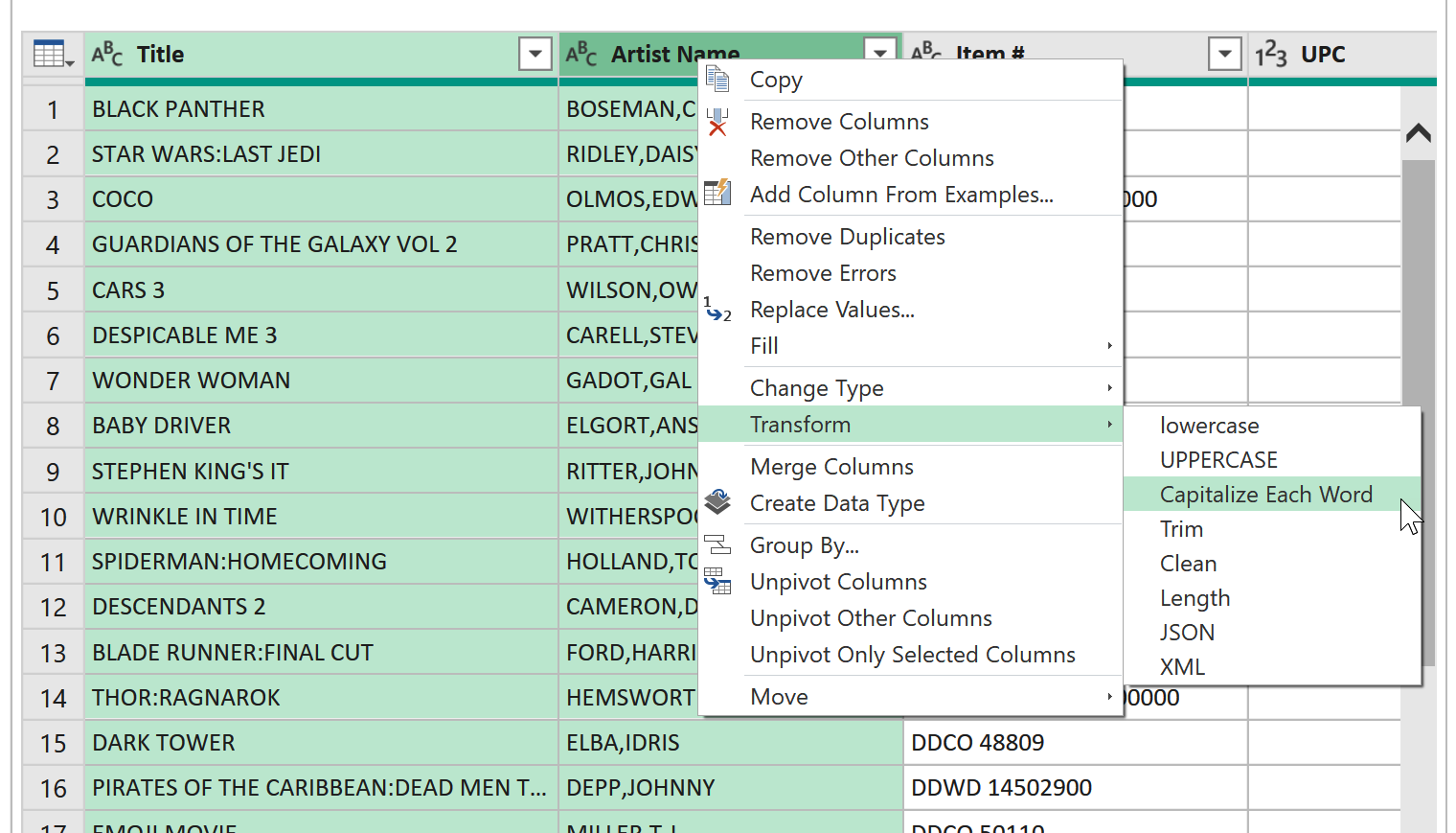
Figure 4-1. Changing text case in Power Query

Notice that Title and Artist Name lack spaces after colons and commas. To address this, with both columns still selected, right-click on either column and choose Replace Values. In the Replace Values dialog box, search for “:” and replace it with a colon followed by a space, as shown in Figure 4-2.

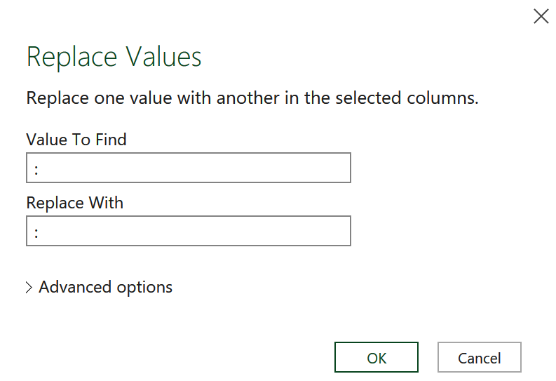
Figure 4-2. Replacing values in Power Query

Next, apply the same process to commas: replace them with a comma followed by a space.

As demonstrated in Chapter 3, Power Query captures every step you perform on the data in the Applied Steps list. This feature greatly facilitates the auditing of text changes compared to the conventional find and replace process.

Delimiting by Column

In Chapter 3, you learned how to split comma-delimit text into rows. Now it’s time to do the same with columns. Right-click on the Item # column and split it into two by selecting Split Column → By Delimiter. In the dialog box, select Space from the drop-down and click OK. Once again, this process offers improved user-friendliness and a broader range of features compared to the traditional Text to Columns function.

The delimited columns are initially labeled as Item #.1 and Item #.2. To rename them, simply double-click on the column headers in the Editor. As with all modifications in Power Query, these alterations are recorded via Applied Steps, allowing for effortless reversal or adjustment as needed.

Changing Data Types

In Power Query, each column is assigned a specific data type, which defines the operations that can be performed on it. When importing a dataset, Power Query automatically tries to determine the most appropriate data type for each column. However, there are situations where this automatic detection can be enhanced or adjusted.

For example, take the UPC column. By default, it is assigned the Whole Number data type. However, since we don’t anticipate conducting significant mathematical operations on this column, it’s more suitable to store it as text. To do this, click the number icon next to the UPC column and change its data type to Text, as seen in Figure 4-3.

Proceed with the following data type changes:

• Convert the ISBN 13 column to Text.

• Convert the Retail column to Currency.

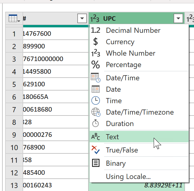
Figure 4-3. Changing column data types in Power Query

Deleting Columns

Removing unnecessary columns from a dataset makes it easier to process and analyze. Select the BTkey column and press the Delete key to remove it from your query. If you decide to include this column later, you can easily retrieve it through the Applied Steps list, as explained in Chapter 2.

Working with Dates

Power Query offers an extensive array of sophisticated methods for managing, transforming, and formatting dates. It facilitates the modification of date types, allowing users to extract components such as the month number and day name, and then store these components in the most appropriate data types.

To explore this functionality, let’s apply it to the Release Date column in a few different ways. Begin by creating copies of this column: right-click on the column and choose “Duplicate Column.” Perform this operation two more times to generate a total of three duplicate date columns.

Right-click the first duplicated Release Date column and navigate to Transform → Year → Year, as in Figure 4-4. The column will be reformatted and its type changed to display only the year instead of the complete date.

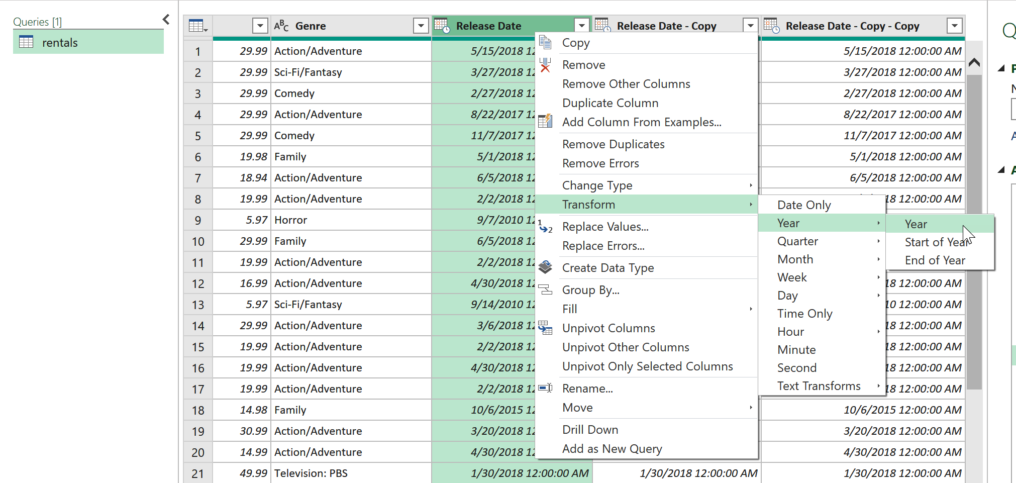
Figure 4-4. Transforming date columns in Power Query

Extract the month and day numbers from the next two columns. Double-click the column headers and rename them as Year, Month, and Day, respectively, to reflect the reformatted data. Close and load your results to an Excel table.

Great job on successfully executing a series of column-oriented data manipulations in Power Query. You’re all set to load this query into Excel.

Creating Custom Columns

Adding a calculated column is a common task in data cleaning. Whether it’s a profit margin, date duration, or something else, Power Query handles this process through its M programming language.

For this next demonstration, head to the teams worksheet of ch_04.xlsx. This dataset includes season records for every Major League Baseball team since 2000. Our objective is to create a new column that calculates the win record for each team during the season. This calculation is done by dividing the number of wins by the total number of wins and losses combined.

The first step, of course, is to load the data into Power Query. Then from the ribbon of the Editor, head to Add Column → Custom Column. Name your custom column Wpct and define it using the following formula:

[W] / ([W] + [L])

The M programming language of Power Query follows a syntax resembling Excel tables, where column references are enclosed in single square brackets. Take advantage of Microsoft’s IntelliSense to hit tab and automatically complete the code as you type these references. Additionally, you have the option to double-click on the desired columns from the “Available columns” list, which will insert them into the formula area.

If everything is correct, a green checkmark will appear at the bottom of the dialog box, indicating that no syntax errors have been detected, as shown in Figure 4-5.

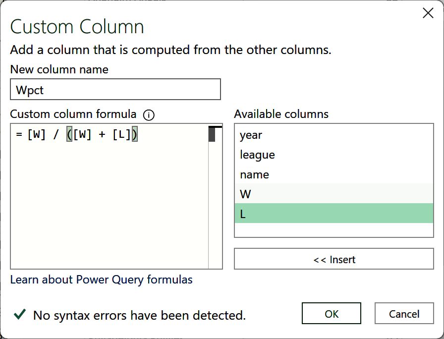
Figure 4-5. Creating a winning percentage calculation

Once you have created this column, go ahead and change its data type in Power Query to Percentage.

Loading & Inspecting the Data

Our new column is calculated and ready to work with. On the Power Query Editor ribbon, head to Home → Close & Load → Close & Load To, then select PivotTable Report and OK. From there, you can analyze the data, such as calculating the average Wpct for each team name, as shown in Figure 4-6.

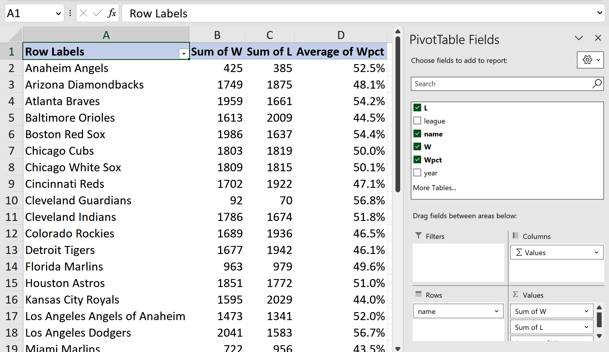
Figure 4-6. Summarizing the results in a PivotTable

Power Query Data Types Versus Excel Cell Formatting

Keep in mind that altering the data type of a column in Power Query only modifies how it’s stored in Power Query itself; it doesn’t change the data’s front-end formatting in Excel. For instance, if you format a column as a percentage in Power Query such as Wpct in the previous example, you’ll still need to apply percentage formatting in Excel itself. In Part III, we’ll explore how to consistently change the data’s presentation through data formatting in Power Pivot.

Calculated Columns Versus Measures

It is important to note that the average Wpct displayed in the PivotTable is a simple, unweighted average of the season’s winning percentages. This means that seasons with a lower number of games—such as the pandemic-affected 2020 season—have a disproportionate impact on the calculation. To verify this, compare the Average of Wpct value in the PivotTable with our own Excel calculation, as shown in Figure 4-7.

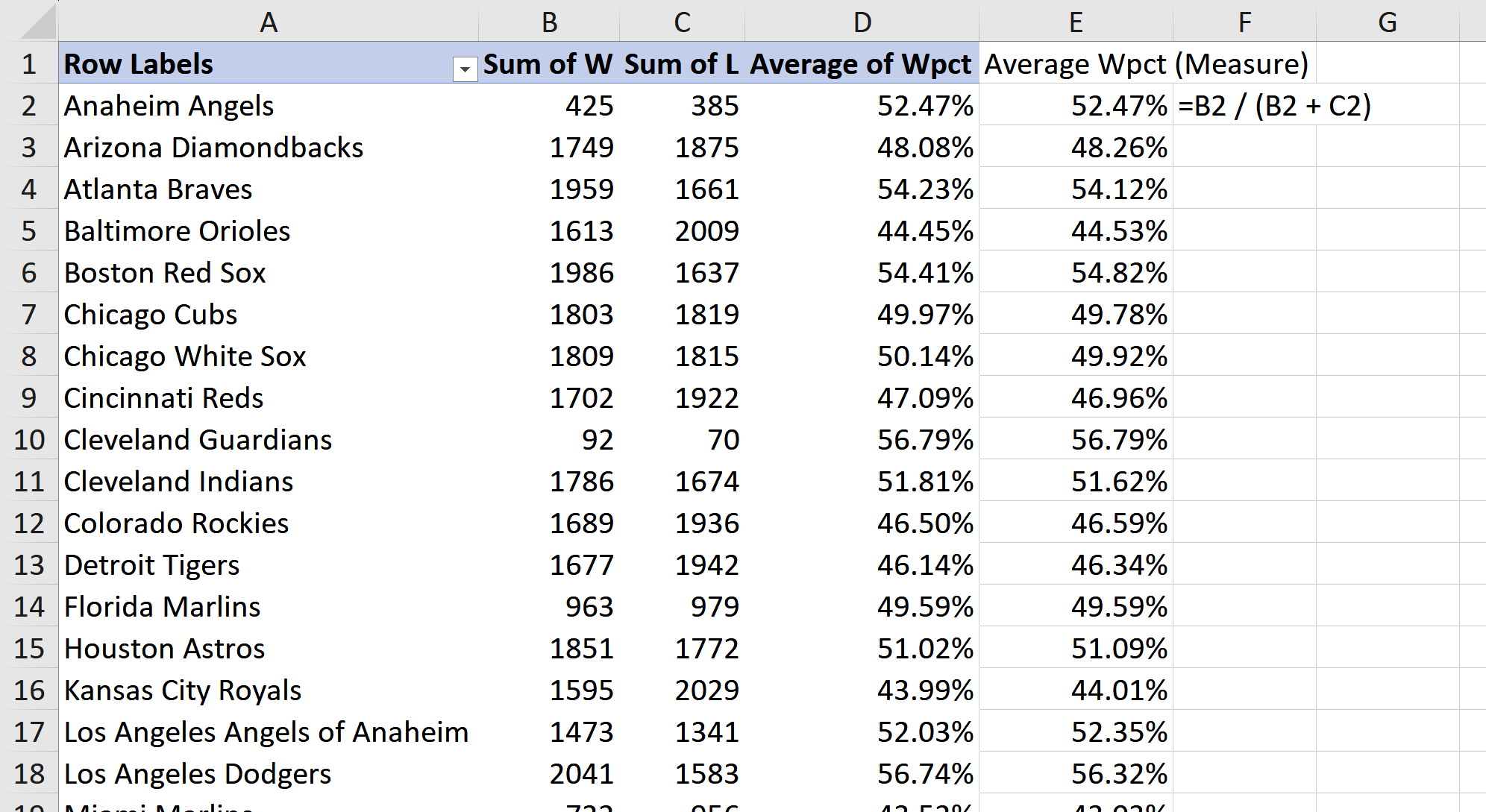
Figure 4-7. Apparent PivotTable miscalculation

To address this issue, one approach involves using dynamic measures for real-time aggregation and calculations tailored to the analysis context. This is achieved with tools such as Power Pivot’s Data Model and the DAX language, discussed in Part II of this book.

This doesn’t mean that calculated columns in Power Query should be avoided altogether. They are simple to create and computationally efficient. Nevertheless, if there is a possibility that these columns might lead to misleading aggregations, it is advisable to opt for a DAX measure instead.

Reshaping Data

In Chapter 1, you were introduced to the concept of “tidy” data, where every variable is stored in one and only one column. You may recall the data in the sales worksheet as an example of untidy data. Fortunately, Power Query resolves this critical data storage problem. To begin, navigate to the familiar sales worksheet of the ch_04.xlsx workbook. Load this table into Power Query to initiate the data transformation process.

The goal is to “unpivot” or “melt” the all sales columns into one column named sales, along with the labels for those sales in one column called department. To do so, hold down the Ctrl key and select the first three variables: customer_id, channel, and region. Right-click and select Unpivot Other Columns, as shown in Figure 4-8.

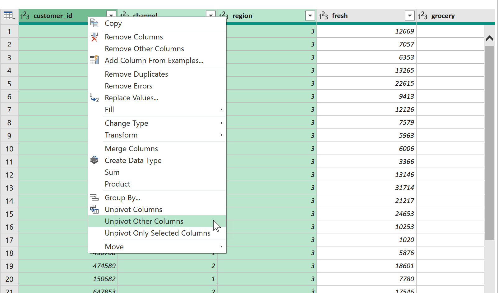
Figure 4-8. Unpivoting a dataset in Power Query

By default, the two resulting unpivoted columns will be called Attribute and Value. Rename them department and sales, respectively. You can now load the query to a PivotTable and analyze sales by channel and region. The results and benefits of creating a PivotTable based on this reshaped data are seen in Figure 4-9.

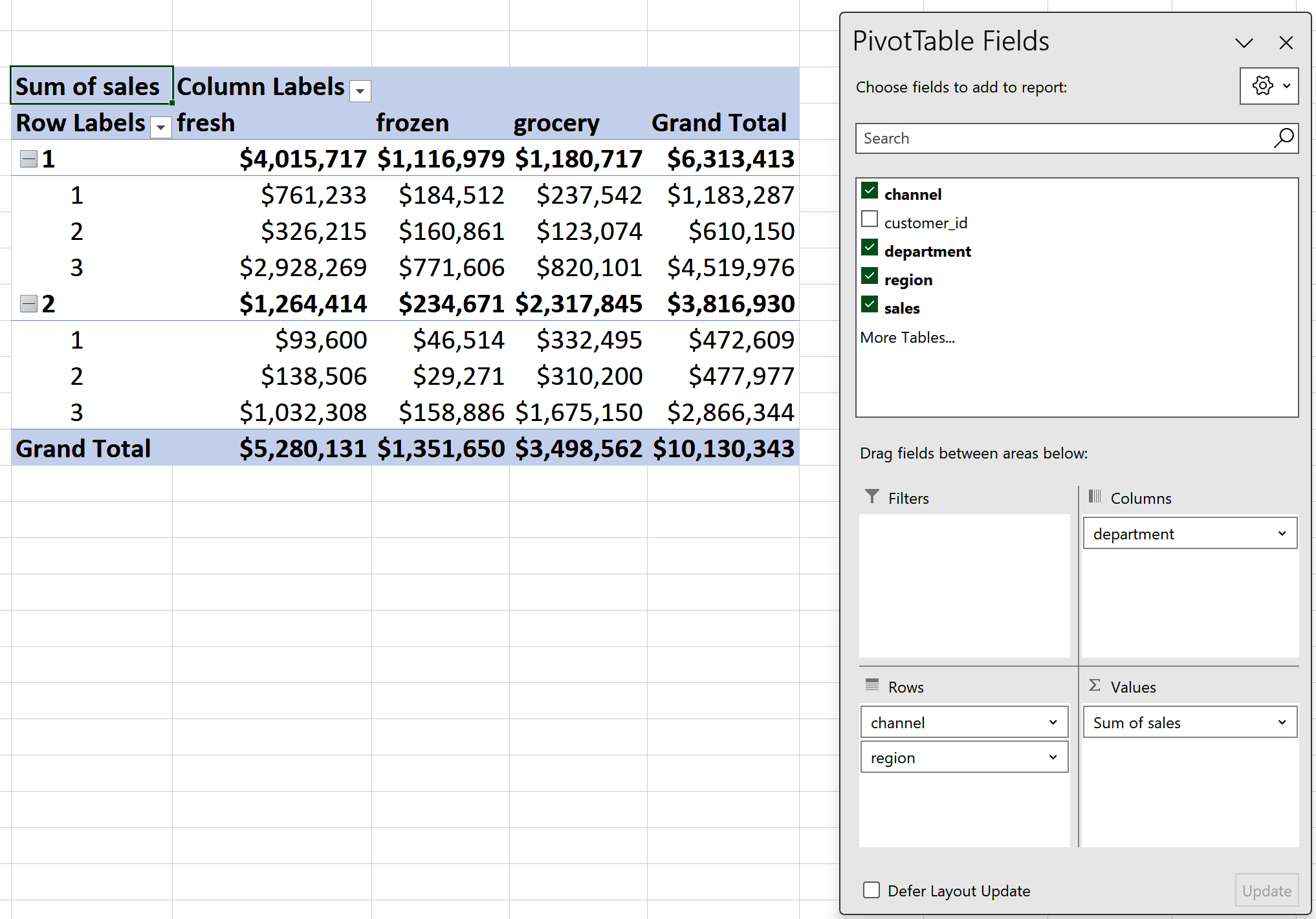
Figure 4-9. Operating on an unpivoted dataset with PivotTables

Conclusion

This chapter explored different ways to manipulate columns in Power Query. Chapter 5 takes a step further by working with multiple datasets in a single query. You’ll learn how to merge and append data sources, as well as how to connect to external sources like .csv files.

Exercises

Practice transforming columns in Power Query with the ch_04_exercises.xlsx file found in the exercises\ch_04_exercises folder in the book’s companion repository. Perform the following transformations to this work orders dataset:

1. Transform the date column to a month format, such as changing 1/1/2023 to January.

2. Transform the owner column to proper case.

3. Split the location column into two separate columns: zip and state.

4. Reshape the dataset so that subscription_cost, support_cost, and services_cost are consolidated into two columns: category and cost.

5. Introduce a new column named tax that calculates 7% of the values in the cost column.

6. Convert the zip variable to the Text data type, and update both cost and tax columns to Currency.

7. Load the results to a table.

For the solutions to these transformations, refer to ch_04_solutions.xlsx in the same folder.