Modern Data Analytics in Excel

Chapter 1. Tables: The Portal to Modern Excel

Excel boasts an extensive array of analytical tools, which can make it challenging to determine the best starting point. However, a fundamental step is mastering the Excel table. This chapter delves into the essential elements of Excel tables, acting as a conduit to Power Query, Power Pivot, and additional tools highlighted in this book. It further underscores the significance of organizing data within a table meticulously. To engage with this chapter’s content, navigate to ch_01.xlsx in the ch_01 folder located within the companion repository of the book.

Creating and Referring to Table Headers

A dataset without column headers is practically useless, as it lacks meaningful context for interpreting what each column measures. Unfortunately, it’s not uncommon to encounter datasets that break this cardinal rule. Excel tables act as a valuable reminder that the quality of a dataset hinges on the presence of clear and informative headers.

In the start worksheet of ch_01.xlsx, you will come across data in columns A:F without corresponding headers, which are currently located in columns H:M. This design is far less than optimal. To adjust it, click anywhere within the primary data source and proceed from the ribbon to Insert → Table → OK, as illustrated in Figure 1-1. Alternatively, you can press Ctrl+T or Ctrl+L from within the data source to launch the same Create Table dialog box.

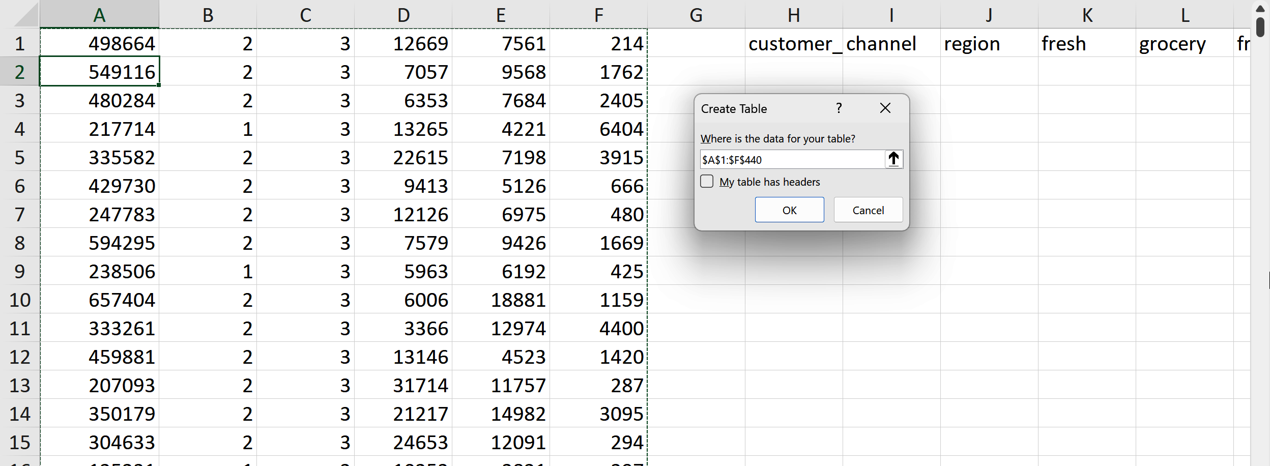
Figure 1-1. Converting the data source into a table

The Create Table dialog box automatically prompts you to specify if your data includes headers. Currently, it does not. In the absence of headers, the dataset is automatically assigned a series of header columns named Column1, Column2, and so forth.

From here, you can cut and paste the headers from columns H:M into the main table to clarify what is being measured in each column, such as in Figure 1-2.

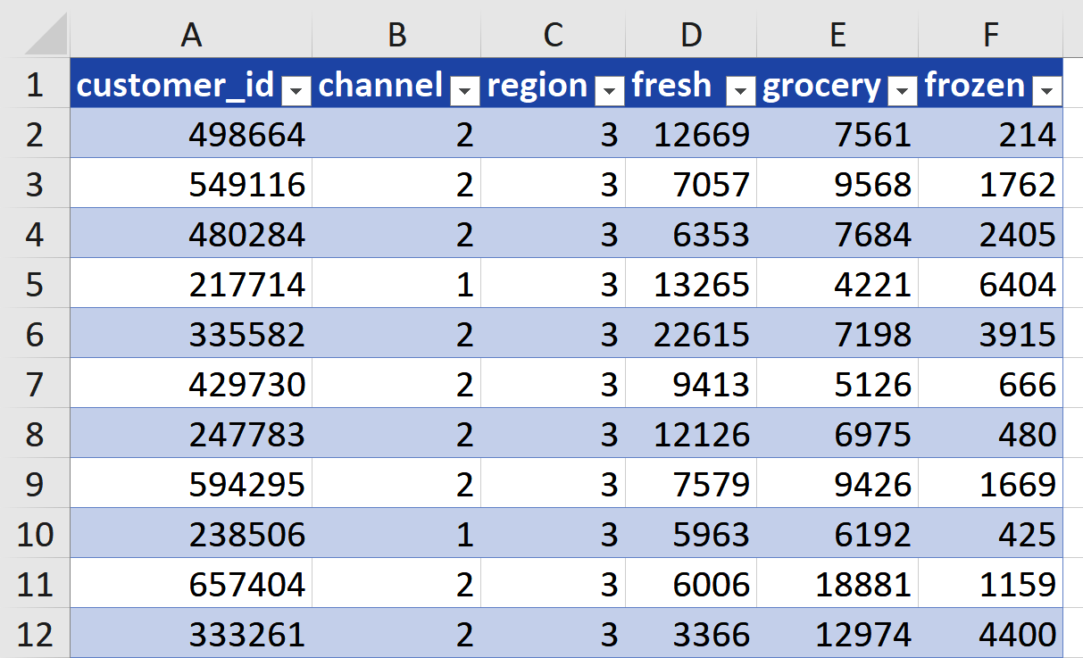
Figure 1-2. Excel table with headers

Header columns in Excel tables occupy a unique role in the dataset. While part of the table, they function as metadata rather than data itself. Excel tables provide the ability to programmatically distinguish between headers and data, unlike classic Excel formulas.

To see this difference in action, head to a blank cell in your worksheet and enter the equals sign. Point to cells A1:F1 as your reference, and you’ll notice that the formula becomes Table1[#Headers].

You can also utilize this reference in other functions. For example, you can use UPPER() to dynamically convert the case of all the headers, such as in Figure 1-3.

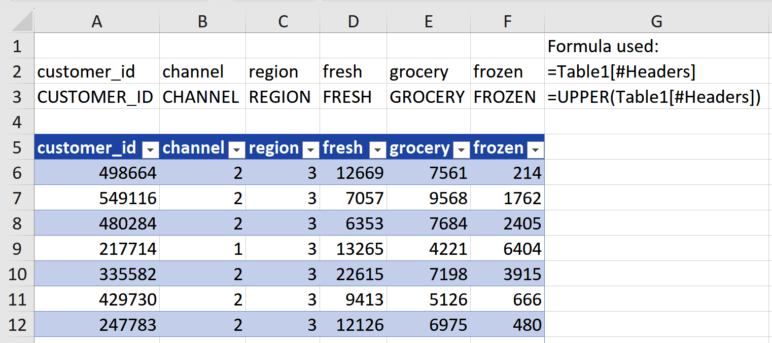
Figure 1-3. Excel header reference formulas

Viewing the Table Footers

Just as every story has a beginning, middle, and end, every Excel table comprises headers, data, and footers. However, footers need to be manually enabled. To do this, click anywhere in the table, navigate to Table Design on the ribbon, and select Total Row in the Table Style Options group, as in Figure 1-4.

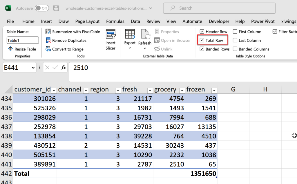
Figure 1-4. Adding footers to a table

By default, the Total Row in a table will calculate the sum of the last column in your data; in this case, frozen. However, you can customize this by clicking the drop-down menu on any column’s footer. For instance, you can find the maximum sales amount of the fresh category, as in Figure 1-5.

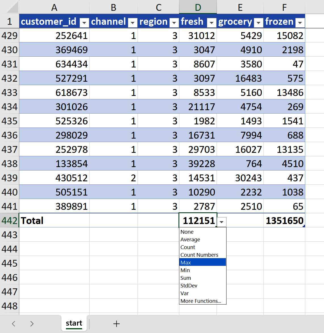
Figure 1-5. Customizing the footers of an Excel table

Table 1-1 summarizes the key formula references for the major components of Excel tables, assuming the table is named Table1.

Table 1-1. Summary of Excel table formula references

Formula	What it refers to
=Table1[#Headers]	Table headers
=Table1	Table data
=Table1[#Totals]	Table footers
=Table1[#All]	Table headers, data, and footers

As you progress in your Excel table skills, you’ll discover additional helpful formula references that rely on the fundamental structure of headers, body, and footers.

Naming Excel Tables

Excel tables offer the advantage of enforcing the use of named ranges, which promotes a more structured approach to working with data. Although referring to Table1 is an improvement over using cell coordinates like A1:F22, it is better to choose a descriptive name that reflects what the data represents.

To accomplish this, go to the Formulas tab on the ribbon, select Name Manager in the Defined Names group, and choose Edit for the Table1 name. Change the name to sales, and then click OK. Figure 1-6 shows what your Name Manager should look like after making this change.

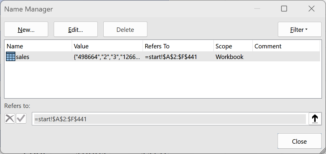
Figure 1-6. Name Manager in Excel

Once you close the Name Manager, you’ll notice that all references to Table1 have been automatically updated to reflect the new name: sales.

Formatting Excel Tables

As an Excel user, you know the importance of presenting data in an appealing format. Tables can be a game changer, instantly enhancing the visual appeal of your worksheet. With tables, you can easily add banded rows, colored headers, and more. To customize the look and feel of your table, click anywhere inside your table and head to Table Design in the ribbon. Take a look at Figure 1-7 for various options, such as changing table colors or toggling Banded Rows on and off.

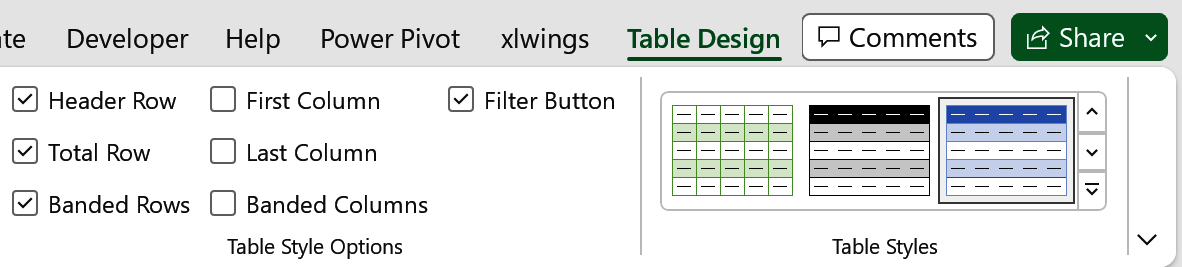
Figure 1-7. Table Design customization options

Updating Table Ranges

With Excel tables, the issue of totals becoming incorrect when data is added or removed is effectively resolved. Thanks to the use of structured references, formulas adapt seamlessly to changes in the data, ensuring accuracy. Furthermore, the total at the bottom of the table is automatically updated to reflect these changes, and it can be easily excluded from external references, maintaining the integrity of your calculations.

Calculate the sum of the fresh column using the structured formula =SUM(sales[fresh]). Microsoft’s IntelliSense facilitates this process by allowing you to complete names efficiently as you type. Experiment with adding or removing rows, or modifying the fresh data in the sales table. You’ll observe that the function to calculate total fresh sales updates dynamically and maintains consistent accuracy.

Referring to data by name instead of cell location minimizes potential formula issues arising from changing the table’s size and placement. Tables also become crucial in preventing problems like missing data in a PivotTable when new rows are added.

Organizing Data for Analytics

While tables are valuable, an even more significant aspect of ensuring effortless and accurate data analysis lies in storing data in the appropriate shape.

Examine the sales table as an example. When attempting to create a PivotTable to calculate total sales by region, the format in which the data is stored presents a challenge. Ideally, all sales information should be consolidated into a single column. However, in the current setup, there is a distinct sales column for each department: fresh, grocery, and frozen. Excel does not recognize that these columns all represent the same metric, namely sales.

The reason this and many other datasets get difficult to analyze is that they are not stored in a format conducive to analysis. The rules of tidy data offer a solution. While Hadley Wickham offers three rules in his 2014 paper by the same name, this book focuses on the first: each variable forms a column.

The sales dataset violates the rule of tidy data by having multiple entries for the same variable, field, across different departments within each row. A helpful rule of thumb is that if multiple columns are measuring the same thing, the data is likely not tidy. By transforming the data into a tidy format, analysis becomes significantly simpler.

In Figure 1-8, you can see a comparison of the dataset before and after the transformation, highlighting the improved tidiness and ease of analysis. In Chapter 4, you will learn how to perform this fundamental transformation on a dataset with just a few clicks. In the meantime, you can explore the sales-tidy worksheet available in ch01_solutions.xlsx, which has already been transformed. Take a look to see firsthand how much simpler it is to obtain total sales by region now.

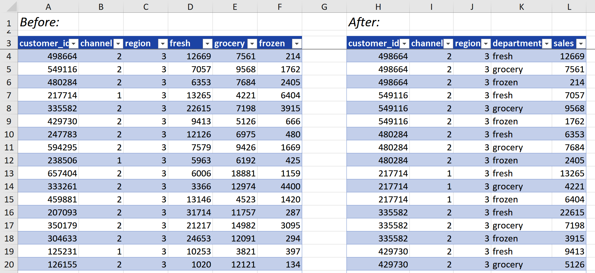
Figure 1-8. Wholesale customers, before and after tidying

Conclusion

This chapter has laid the groundwork for utilizing Excel tables effectively. For an in-depth exploration of maximizing the potential of tables, including the application of structured references to formulate calculated columns, refer to Excel Tables: A Complete Guide for Creating, Using, and Automating Lists and Tables by Zack Barresse and Kevin Jones (Holy Macro! Books, 2014). Additionally, this chapter delved into the meticulous organization of data, a fundamental aspect of any successful data analysis project in Excel. Chapter 2 offers an introduction to simplifying data transformation with Power Query.

Exercises

To create, analyze, and manipulate data in Excel tables, follow the exercises using the penguins dataset located in ch_01_exercises.xlsx in the exercises\ch_01_exercises folder in the book’s companion repository:

1. Convert the data to a table named penguins.

2. Utilize a formula reference to capitalize each column header.

3. Generate a new column called bill_ratio by dividing bill_length_mm by bill_depth_mm.

4. Include a total row to calculate the average body_mass_g.

5. Remove the banded row styling from the table.

For the solutions, refer to the ch_01_exercise_solutions.xlsx file located in the same folder.