Essential Math for Data Science

Chapter 4. Linear Algebra

Changing gears a little bit, let’s venture away from probability and statistics and into linear algebra. Sometimes people confuse linear algebra with basic algebra, thinking maybe it has to do with plotting lines using the algebraic function y = mx + b. This is why linear algebra probably should have been called “vector algebra” or “matrix algebra” because it is much more abstract. Linear systems play a role but in a much more metaphysical way.

So, what exactly is linear algebra? Well, linear algebra concerns itself with linear systems but represents them through vector spaces and matrices. If you do not know what a vector or a matrix is, do not worry! We will define and explore them in depth. Linear algebra is hugely fundamental to many applied areas of math, statistics, operations research, data science, and machine learning. When you work with data in any of these areas, you are using linear algebra and perhaps you may not even know it.

You can get away with not learning linear algebra for a while, using machine learning and statistics libraries that do it all for you. But if you are going to get intuition behind these black boxes and be more effective at working with data, understanding the fundamentals of linear algebra is inevitable. Linear algebra is an enormous topic that can fill thick textbooks, so of course we cannot gain total mastery in just one chapter of this book. However, we can learn enough to be more comfortable with it and navigate the data science domain effectively. There will also be opportunities to apply it in the remaining chapters in this book, including Chapters 5 and 7.

What Is a Vector?

Simply put, a vector is an arrow in space with a specific direction and length, often representing a piece of data. It is the central building block of linear algebra, including matrices and linear transformations. In its fundamental form, it has no concept of location so always imagine its tail starts at the origin of a Cartesian plane (0,0).

Figure 4-1 shows a vector $\overrightarrow{v}$ that moves three steps in the horizontal direction and two steps in the vertical direction.

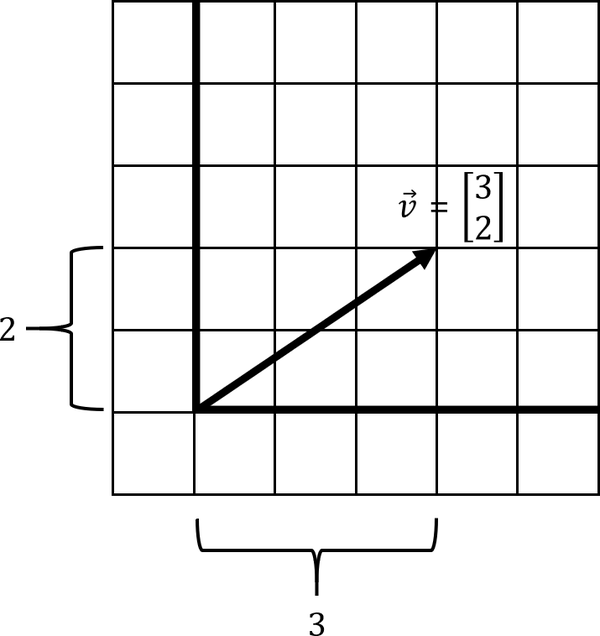
Figure 4-1. A simple vector

To emphasize again, the purpose of the vector is to visually represent a piece of data. If you have a data record for the square footage of a house 18,000 square feet and its valuation $260,000, we could express that as a vector [18000, 260000], stepping 18,000 steps in the horizontal direction and 260,000 steps in the vertical direction.

We declare a vector mathematically like this:

$$\begin{array}{c}\hfill \overrightarrow{v}=\left[\begin{array}{c}x\\ y\end{array}\right]\\ \\ \end{array}$$$$\begin{array}{c}\hfill \overrightarrow{v}=\left[\begin{array}{c}3\\ 2\end{array}\right]\end{array}$$

We can declare a vector using a simple Python collection, like a Python list as shown in Example 4-1.

Example 4-1. Declaring a vector in Python using a list

v = [3, 2]
print(v)

However, when we start doing mathematical computations with vectors, especially when doing tasks like machine learning, we should probably use the NumPy library as it is more efficient than plain Python. You can also use SymPy to perform linear algebra operations, and we will use it occasionally in this chapter when decimals become inconvenient. However, NumPy is what you will likely use in practice so that is what we will mainly stick to.

To declare a vector, you can use NumPy’s array() function and then can pass a collection of numbers to it as shown in Example 4-2.

Example 4-2. Declaring a vector in Python using NumPy

import numpy as np
v = np.array([3, 2])
print(v)

Python Is Slow, Its Numerical Libraries Are Not

Python is a computationally slow language platform, as it does not compile to lower-level machine code and bytecode like Java, C#, C, etc. It is dynamically interpreted at runtime. However, Python’s numeric and scientific libraries are not slow. Libraries like NumPy are typically written in low-level languages like C and C++, hence why they are computationally efficient. Python really acts as “glue code” integrating these libraries for your tasks.

A vector has countless practical applications. In physics, a vector is often thought of as a direction and magnitude. In math, it is a direction and scale on an XY plane, kind of like a movement. In computer science, it is an array of numbers storing data. The computer science context is the one we will become the most familiar with as data science professionals. However, it is important we never forget the visual aspect so we do not think of vectors as esoteric grids of numbers. Without a visual understanding, it is almost impossible to grasp many fundamental linear algebra concepts like linear dependence and determinants.

Here are some more examples of vectors. In Figure 4-2 note that some of these vectors have negative directions on the X and Y scales. Vectors with negative directions will have an impact when we combine them later, essentially subtracting rather than adding them together.

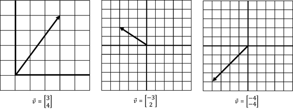
Figure 4-2. A sampling of different vectors

Why Are Vectors Useful?

A struggle many people have with vectors (and linear algebra in general) is understanding why they are useful. They are a highly abstract concept but they have many tangible applications. Computer graphics are easier to work with when you have a grasp of vectors and linear transformations (the fantastic Manim visualization library defines animations and transformations with vectors). When doing statistics and machine learning work, data is often imported and turned into numerical vectors so we can work with it. Solvers like the one in Excel or Python PuLP use linear programming, which uses vectors to maximize a solution while meeting those constraints. Even video games and flight simulators use vectors and linear algebra to model not just graphics but also physics. I think what makes vectors so hard to grasp is not that their application is unobvious, but rather these applications are so diverse it is hard to see the generalization.

Note also vectors can exist on more than two dimensions. Next we declare a three-dimensional vector along axes x, y, and z:

$$\overrightarrow{v}=\left[\begin{array}{c}x\\ y\\ z\end{array}\right]=\left[\begin{array}{c}4\\ 1\\ 2\end{array}\right]$$

To create this vector, we are stepping four steps in the x direction, one in the y direction, and two in the z direction. Here it is visualized in Figure 4-3. Note that we no longer are showing a vector on a two-dimensional grid but rather a three-dimensional space with three axes: x, y, and z.

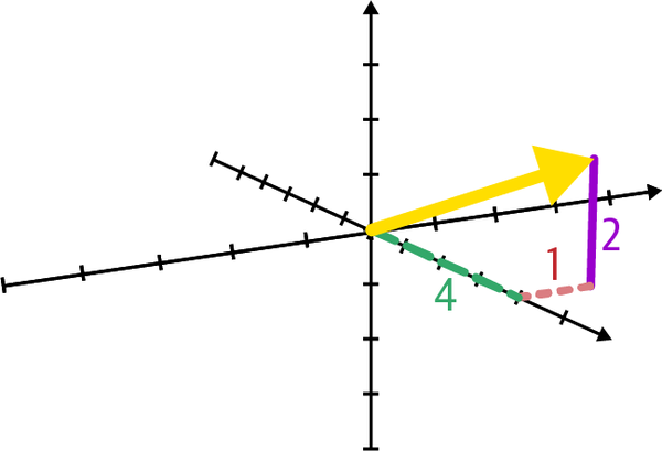
Figure 4-3. A three-dimensional vector

Naturally, we can express this three-dimensional vector in Python using three numeric values, as declared in Example 4-3.

Example 4-3. Declaring a three-dimensional vector in Python using NumPy

import numpy as np
v = np.array([4, 1, 2])
print(v)

Like many mathematical models, visualizing more than three dimensions is challenging and something we will not expend energy doing in this book. But numerically, it is still straightforward. Example 4-4 shows how we declare a five-dimensional vector mathematically in Python.

$$\overrightarrow{v}=\left[\begin{array}{c}6\\ 1\\ 5\\ 8\\ 3\end{array}\right]$$

Example 4-4. Declaring a five-dimensional vector in Python using NumPy

import numpy as np
v = np.array([6, 1, 5, 8, 3])
print(v)

Adding and Combining Vectors

On their own, vectors are not terribly interesting. You express a direction and size, kind of like a movement in space. But when you start combining vectors, known as vector addition, it starts to get interesting. We effectively combine the movements of two vectors into a single vector.

Say we have two vectors $\overrightarrow{v}$ and $\overrightarrow{w}$ as shown in Figure 4-4. How do we add these two vectors together?

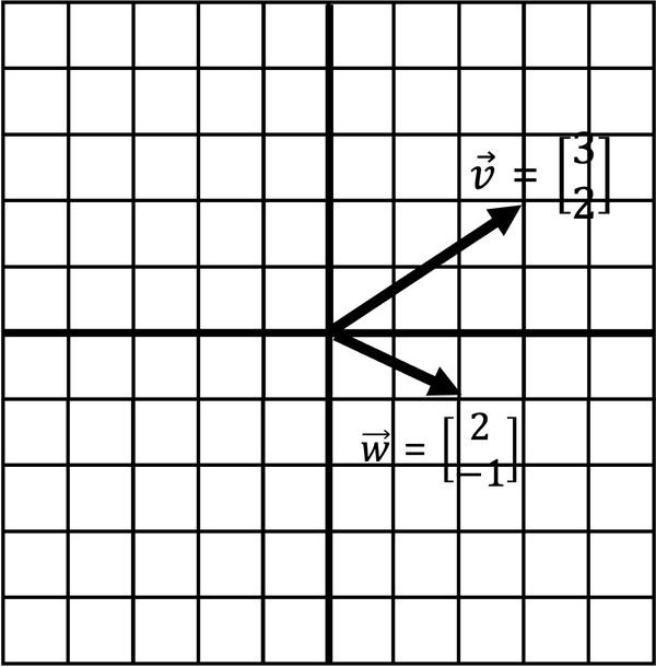
Figure 4-4. Adding two vectors together

We will get to why adding vectors is useful in a moment. But if we wanted to combine these two vectors, including their direction and scale, what would that look like? Numerically, this is straightforward. You simply add the respective x-values and then the y-values into a new vector as shown in Example 4-5.

$$\begin{array}{c}\hfill \overrightarrow{v}=\left[\begin{array}{c}3\\ 2\end{array}\right]\\ \\ \\ \end{array}$$$$\begin{array}{c}\hfill \overrightarrow{w}=\left[\begin{array}{c}2\\ -1\end{array}\right]\\ \\ \\ \end{array}$$$$\begin{array}{c}\hfill \overrightarrow{v}+\overrightarrow{w}=\left[\begin{array}{c}3+2\\ 2+-1\end{array}\right]=\left[\begin{array}{c}5\\ 1\end{array}\right]\end{array}$$

Example 4-5. Adding two vectors in Python using NumPy

from numpy import array

v = array([3,2])
w = array([2,-1])

# sum the vectors
v_plus_w = v + w

# display summed vector
print(v_plus_w) # [5, 1]

But what does this mean visually? To visually add these two vectors together, connect one vector after the other and walk to the tip of the last vector (Figure 4-5). The point you end at is a new vector, the result of summing the two vectors.

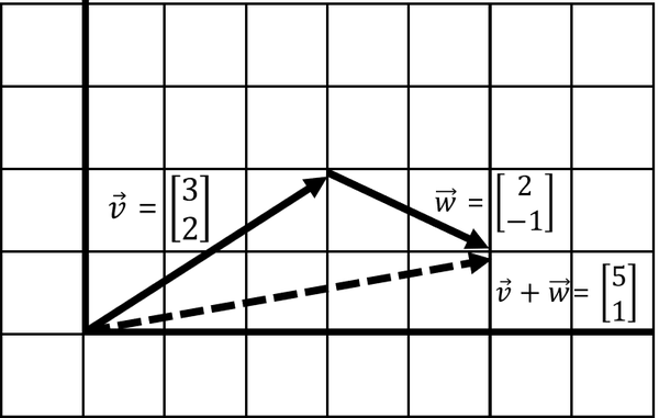
Figure 4-5. Adding two vectors into a new vector

As seen in Figure 4-5, when we walk to the end of the last vector $\overrightarrow{w}$ we end up with a new vector [5, 1]. This new vector is the result of summing $\overrightarrow{v}$ and $\overrightarrow{w}$. In practice, this can be simply adding data together. If we were totaling housing values and their square footage in an area, we would be adding several vectors into a single vector in this manner.

Note that it does not matter whether we add $\overrightarrow{v}$ before $\overrightarrow{w}$ or vice versa, which means it is commutative and order of operation does not matter. If we walk $\overrightarrow{w}$ before $\overrightarrow{v}$ we end up with the same resulting vector [5, 1] as visualized in Figure 4-6.

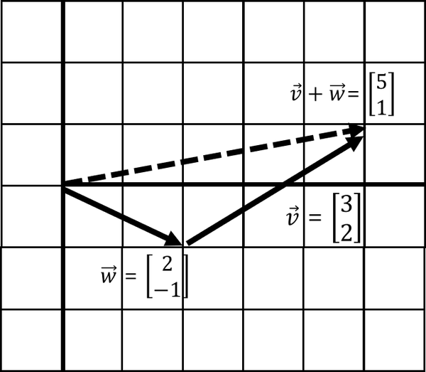
Figure 4-6. Adding vectors is commutative

Scaling Vectors

Scaling is growing or shrinking a vector’s length. You can grow/shrink a vector by multiplying or scaling it with a single value, known as a scalar. Figure 4-7 is vector $\overrightarrow{v}$ being scaled by a factor of 2, which doubles it.

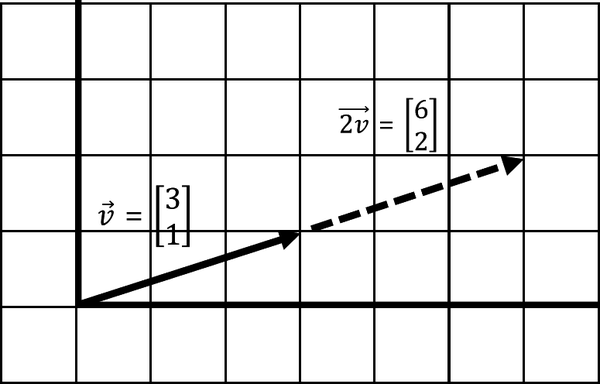
Figure 4-7. Scaling a vector

Mathematically, you multiply each element of the vector by the scalar value:

$$\begin{array}{c}\hfill \overrightarrow{v}=\left[\begin{array}{c}3\\ 1\end{array}\right]\\ \\ \\ \end{array}$$$$\begin{array}{c}\hfill 2\overrightarrow{v}=2\left[\begin{array}{c}3\\ 1\end{array}\right]=\left[\begin{array}{c}3\times 2\\ 1\times 2\end{array}\right]=\left[\begin{array}{c}6\\ 2\end{array}\right]\end{array}$$

Performing this scaling operation in Python is as easy as multiplying a vector by the scalar, as coded in Example 4-6.

Example 4-6. Scaling a number in Python using NumPy

from numpy import array

v = array([3,1])

# scale the vector
scaled_v = 2.0 * v

# display scaled vector
print(scaled_v) # [6 2]

Here in Figure 4-8 $\overrightarrow{v}$ is being scaled down by factor of .5, which halves it.

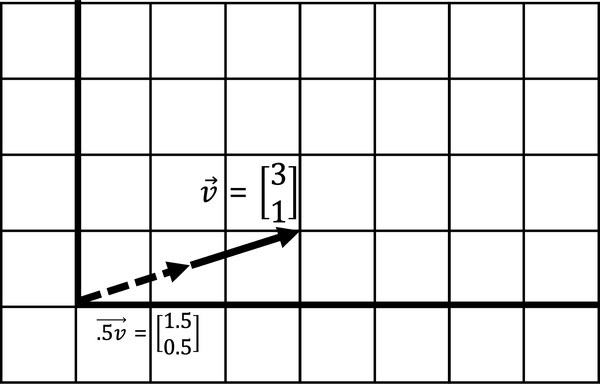
Figure 4-8. Scaling down a vector by half

Manipulating Data Is Manipulating Vectors

Every data operation can be thought of in terms of vectors, even simple averages.

Take scaling, for example. Let’s say we were trying to get the average house value and average square footage for an entire neighborhood. We would add the vectors together to combine their value and square footage respectively, giving us one giant vector containing both total value and total square footage. We then scale down the vector by dividing by the number of houses N, which really is multiplying by 1/N. We now have a vector containing the average house value and average square footage.

An important detail to note here is that scaling a vector does not change its direction, only its magnitude. But there is one slight exception to this rule as visualized in Figure 4-9. When you multiply a vector by a negative number, it flips the direction of the vector as shown in the image.

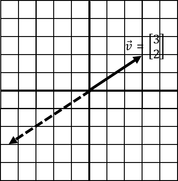
Figure 4-9. A negative scalar flips the vector direction

When you think about it, though, scaling by a negative number has not really changed direction in that it still exists on the same line. This segues to a key concept called linear dependence.

Span and Linear Dependence

These two operations, adding two vectors and scaling them, brings about a simple but powerful idea. With these two operations, we can combine two vectors and scale them to create any resulting vector we want. Figure 4-10 shows six examples of taking two vectors $\overrightarrow{v}$ and $\overrightarrow{w}$, and scaling and combining. These vectors $\overrightarrow{v}$ and $\overrightarrow{w}$, fixed in two different directions, can be scaled and added to create any new vector $\overrightarrow{v+w}$.

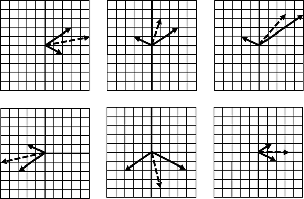
Figure 4-10. Scaling two added vectors allows us to create any new vector

Again, $\overrightarrow{v}$ and $\overrightarrow{w}$ are fixed in direction, except for flipping with negative scalars, but we can use scaling to freely create any vector composed of $\overrightarrow{v+w}$.

This whole space of possible vectors is called span, and in most cases our span can create unlimited vectors off those two vectors, simply by scaling and summing them. When we have two vectors in two different directions, they are linearly independent and have this unlimited span.

But in what case are we limited in the vectors we can create? Think about it and read on.

What happens when two vectors exist in the same direction, or exist on the same line? The combination of those vectors is also stuck on the same line, limiting our span to just that line. No matter how you scale it, the resulting sum vector is also stuck on that same line. This makes them linearly dependent, as shown in Figure 4-11.

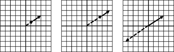
Figure 4-11. Linearly dependent vectors

The span here is stuck on the same line as the two vectors it is made out of. Because the two vectors exist on the same underlying line, we cannot flexibly create any new vector through scaling.

In three or more dimensions, when we have a linearly dependent set of vectors, we often get stuck on a plane in a smaller number of dimensions. Here is an example of being stuck on a two-dimensional plane even though we have three-dimensional vectors as declared in Figure 4-12.

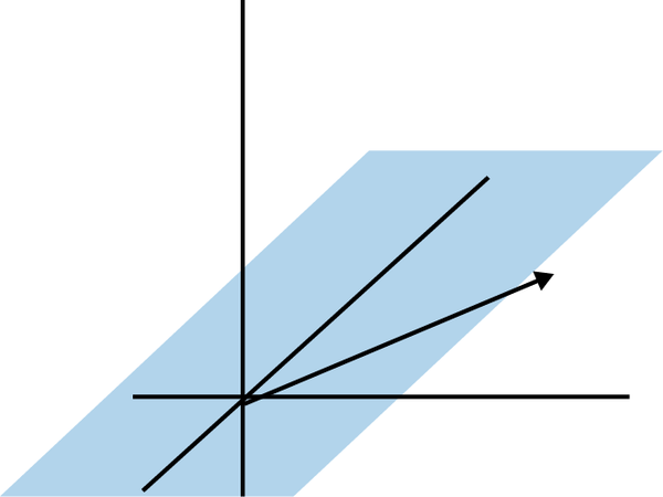
Figure 4-12. Linear dependence in three dimensions; note our span is limited to a flat plane

Later we will learn a simple tool called the determinant to check for linear dependence, but why do we care whether two vectors are linearly dependent or independent? A lot of problems become difficult or unsolvable when they are linearly dependent. For example, when we learn about systems of equations later in this chapter, a linearly dependent set of equations can cause variables to disappear and make the problem unsolvable. But if you have linear independence, that flexibility to create any vector you need from two or more vectors becomes invaluable to solve for a solution!

Linear Transformations

This concept of adding two vectors with fixed direction, but scaling them to get different combined vectors, is hugely important. This combined vector, except in cases of linear dependence, can point in any direction and have any length we choose. This sets up an intuition for linear transformations where we use a vector to transform another vector in a function-like manner.

Basis Vectors

Imagine we have two simple vectors $\widehat{i}$ and $\widehat{j}$ (“i-hat” and “j-hat”). These are known as basis vectors, which are used to describe transformations on other vectors. They typically have a length of 1 and point in perpendicular positive directions as visualized in Figure 4-13.

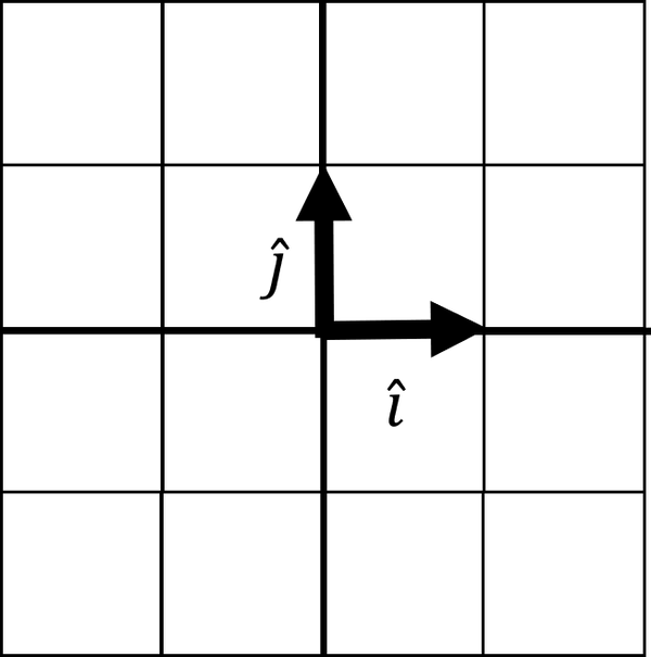
Figure 4-13. Basis vectors $\widehat{i}$ and $\widehat{j}$

Think of the basis vectors as building blocks to build or transform any vector. Our basis vector is expressed in a 2 × 2 matrix, where the first column is $\widehat{i}$ and the second column is $\widehat{j}$:

$$\begin{array}{c}\hfill \widehat{i}=\left[\begin{array}{c}1\\ 0\end{array}\right]\\ \\ \\ \end{array}$$$$\begin{array}{c}\hfill \widehat{j}=\left[\begin{array}{c}0\\ 1\end{array}\right]\\ \\ \\ \end{array}$$$$\begin{array}{c}\hfill \text{basis}=\left[\begin{array}{cc}1& 0\\ 0& 1\end{array}\right]\end{array}$$

A matrix is a collection of vectors (such as $\widehat{i}$, $\widehat{j}$) that can have multiple rows and columns and is a convenient way to package data. We can use $\widehat{i}$ and $\widehat{j}$ to create any vector we want by scaling and adding them. Let’s start with each having a length of 1 and showing the resulting vector $\overrightarrow{v}$ in Figure 4-14.

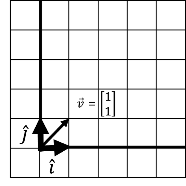
Figure 4-14. Creating a vector from basis vectors

I want vector $\overrightarrow{v}$ to land at [3, 2]. What happens to $\overrightarrow{v}$ if we stretch $\widehat{i}$ by a factor of 3 and $\widehat{j}$ by a factor of 2? First we scale them individually as shown here:

$$\begin{array}{c}\hfill 3\widehat{i}=3\left[\begin{array}{c}1\\ 0\end{array}\right]=\left[\begin{array}{c}3\\ 0\end{array}\right]\\ \\ \\ \end{array}$$$$\begin{array}{c}\hfill 2\widehat{j}=2\left[\begin{array}{c}0\\ 1\end{array}\right]=\left[\begin{array}{c}0\\ 2\end{array}\right]\end{array}$$

If we stretched space in these two directions, what does this do to $\overrightarrow{v}$? Well, it is going to stretch with $\widehat{i}$ and $\widehat{j}$. This is known as a linear transformation, where we transform a vector with stretching, squishing, sheering, or rotating by tracking basis vector movements. In this case (Figure 4-15), scaling $\widehat{i}$ and $\widehat{j}$ has stretched space along with our vector $\overrightarrow{v}$.

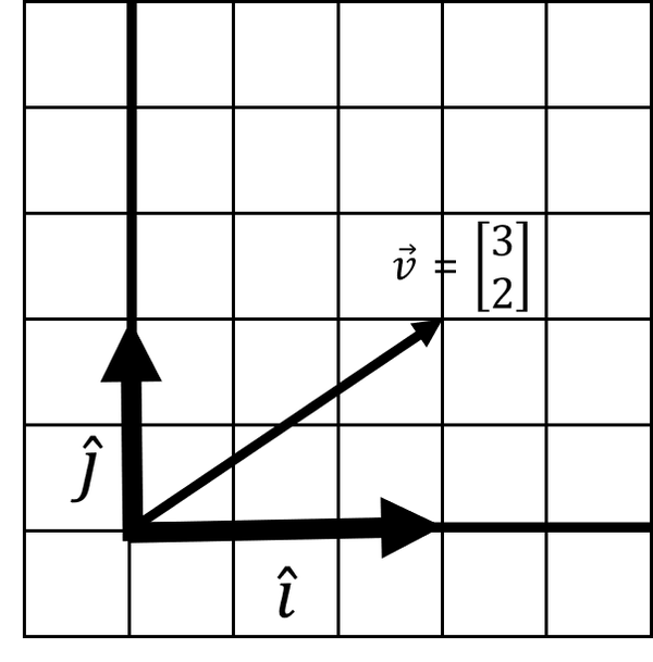
Figure 4-15. A linear transformation

But where does $\overrightarrow{v}$ land? It is easy to see where it lands here, which is [3, 2]. Recall that vector $\overrightarrow{v}$ is composed of adding $\widehat{i}$ and $\widehat{j}$. So we simply take the stretched $\widehat{i}$ and $\widehat{j}$ and add them together to see where vector $\overrightarrow{v}$ has landed:

$${\overrightarrow{v}}_{new}=\left[\begin{array}{c}3\\ 0\end{array}\right]+\left[\begin{array}{c}0\\ 2\end{array}\right]=\left[\begin{array}{c}3\\ 2\end{array}\right]$$

Generally, with linear transformations, there are four movements you can achieve, as shown in Figure 4-16.

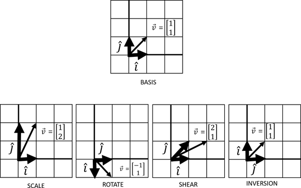
Figure 4-16. Four movements can be achieved with linear transformations

These four linear transformations are a central part of linear algebra. Scaling a vector will stretch or squeeze it. Rotations will turn the vector space, and inversions will flip the vector space so that $\widehat{i}$ and $\widehat{j}$ swap respective places. A shear is easier to describe visually, but it displaces each point in a fixed direction proportionally to its distance from a given line parallel to that direction.

It is important to note that you cannot have transformations that are nonlinear, resulting in curvy or squiggly transformations that no longer respect a straight line. This is why we call it linear algebra, not nonlinear algebra!

Matrix Vector Multiplication

This brings us to our next big idea in linear algebra. This concept of tracking where $\widehat{i}$ and $\widehat{j}$ land after a transformation is important because it allows us not just to create vectors but also to transform existing vectors. If you want true linear algebra enlightenment, think why creating vectors and transforming vectors are actually the same thing. It’s all a matter of relativity given your basis vectors being a starting point before and after a transformation.

The formula to transform a vector $\overrightarrow{v}$ given basis vectors $\widehat{i}$ and $\widehat{j}$ packaged as a matrix is:

$$\begin{array}{c}\hfill \left[\begin{array}{c}{x}_{new}\\ y_{new}\end{array}\right]=\left[\begin{array}{cc}a& b\\ c& d\end{array}\right]\left[\begin{array}{c}x\\ y\end{array}\right]\\ \\ \\ \end{array}$$$$\begin{array}{c}\hfill \left[\begin{array}{c}{x}_{new}\\ y_{new}\end{array}\right]=\left[\begin{array}{c}ax+by\\ cx+dy\end{array}\right]\end{array}$$

$\widehat{i}$ is the first column [a, c] and $\widehat{j}$ is the column [b, d]. We package both of these basis vectors as a matrix, which again is a collection of vectors expressed as a grid of numbers in two or more dimensions. This transformation of a vector by applying basis vectors is known as matrix vector multiplication. This may seem contrived at first, but this formula is a shortcut for scaling and adding $\widehat{i}$ and $\widehat{j}$ just like we did earlier adding two vectors, and applying the transformation to any vector $\overrightarrow{v}$.

So in effect, a matrix really is a transformation expressed as basis vectors.

To execute this transformation in Python using NumPy, we will need to declare our basis vectors as a matrix and then apply it to vector $\overrightarrow{v}$ using the dot() operator (Example 4-7). The dot() operator will perform this scaling and addition between our matrix and vector as we just described. This is known as the dot product, and we will explore it throughout this chapter.

Example 4-7. Matrix vector multiplication in NumPy

from numpy import array

# compose basis matrix with i-hat and j-hat
basis = array(
    [[3, 0],
     [0, 2]]
 )

# declare vector v
v = array([1,1])

# create new vector
# by transforming v with dot product
new_v = basis.dot(v)

print(new_v) # [3, 2]

When thinking in terms of basis vectors, I prefer to break out the basis vectors and then compose them together into a matrix. Just note you will need to transpose, or swap the columns and rows. This is because NumPy’s array() function will do the opposite orientation we want, populating each vector as a row rather than a column. Transposition in NumPy is demonstrated in Example 4-8.

Example 4-8. Separating the basis vectors and applying them as a transformation

from numpy import array

# Declare i-hat and j-hat
i_hat = array([2, 0])
j_hat = array([0, 3])

# compose basis matrix using i-hat and j-hat
# also need to transpose rows into columns
basis = array([i_hat, j_hat]).transpose()

# declare vector v
v = array([1,1])

# create new vector
# by transforming v with dot product
new_v = basis.dot(v)

print(new_v) # [2, 3]

Here’s another example. Let’s start with vector $\overrightarrow{v}$ being [2, 1] and $\widehat{i}$ and $\widehat{j}$ start at [1, 0] and [0, 1], respectively. We then transform $\widehat{i}$ and $\widehat{j}$ to [2, 0] and [0, 3]. What happens to vector $\overrightarrow{v}$? Working this out mathematically by hand using our formula, we get this:

$$\left[\begin{array}{c}{x}_{new}\\ y_{new}\end{array}\right]=\left[\begin{array}{cc}a& b\\ c& d\end{array}\right]\left[\begin{array}{c}x\\ y\end{array}\right]=\left[\begin{array}{c}ax+by\\ cx+dy\end{array}\right]$$

$$\left[\begin{array}{c}{x}_{new}\\ y_{new}\end{array}\right]=\left[\begin{array}{cc}2& 0\\ 0& 3\end{array}\right]\left[\begin{array}{c}2\\ 1\end{array}\right]=\left[\begin{array}{c}\left(2\right)\left(2\right)+\left(0\right)\left(1\right)\\ \left(2\right)\left(0\right)+\left(3\right)\left(1\right)\end{array}\right]=\left[\begin{array}{c}4\\ 3\end{array}\right]$$

Example 4-9 shows this solution in Python.

Example 4-9. Transforming a vector using NumPy

from numpy import array

# Declare i-hat and j-hat
i_hat = array([2, 0])
j_hat = array([0, 3])

# compose basis matrix using i-hat and j-hat
# also need to transpose rows into columns
basis = array([i_hat, j_hat]).transpose()


# declare vector v 0
v = array([2,1])

# create new vector
# by transforming v with dot product
new_v = basis.dot(v)

print(new_v) # [4, 3]

The vector $\overrightarrow{v}$ now lands at [4, 3]. Figure 4-17 shows what this transformation looks like.

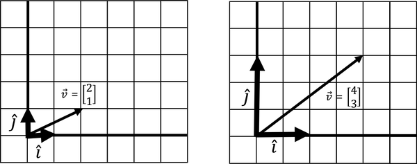
Figure 4-17. A stretching linear transformation

Here is an example that jumps things up a notch. Let’s take vector $\overrightarrow{v}$ of value [2, 1]. $\widehat{i}$ and $\widehat{j}$ start at [1, 0] and [0, 1], but then are transformed and land at [2, 3] and [2, -1]. What happens to $\overrightarrow{v}$? Let’s look in Figure 4-18 and Example 4-10.

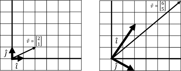
Figure 4-18. A linear transformation that does a rotation, shear, and flipping of space

Example 4-10. A more complicated transformation

from numpy import array

# Declare i-hat and j-hat
i_hat = array([2, 3])
j_hat = array([2, -1])

# compose basis matrix using i-hat and j-hat
# also need to transpose rows into columns
basis = array([i_hat, j_hat]).transpose()

# declare vector v 0
v = array([2,1])

# create new vector
# by transforming v with dot product
new_v = basis.dot(v)

print(new_v) # [6, 5]

A lot has happened here. Not only did we scale $\widehat{i}$ and $\widehat{j}$ and elongate vector $\overrightarrow{v}$. We actually sheared, rotated, and flipped space, too. You know space was flipped when $\widehat{i}$ and $\widehat{j}$ change places in their clockwise orientation, and we will learn how to detect this with determinants later in this chapter.

Basis Vectors in 3D and Beyond

You might be wondering how we think of vector transformations in three dimensions or more. The concept of basis vectors extends quite nicely. If I have a three-dimensional vector space, then I have basis vectors $\widehat{i}$, $\widehat{j}$, and $\widehat{k}$. I just keep adding more letters from the alphabet for each new dimension (Figure 4-19).

Figure 4-19. 3D basis vector

Something else that is worth pointing out is some linear transformations can shift a vector space into fewer or more dimensions, and that is exactly what nonsquare matrices will do (where number of rows and columns are not equal). In the interest of time we cannot explore this. But 3Blue1Brown explains and animates this concept beautifully.

Matrix Multiplication

We learned how to multiply a vector and a matrix, but what exactly does multiplying two matrices accomplish? Think of matrix multiplication as applying multiple transformations to a vector space. Each transformation is like a function, where we apply the innermost first and then apply each subsequent transformation outward.

Here is how we apply a rotation and then a shear to any vector $\overrightarrow{v}$ with value [x, y]:

$$\left[\begin{array}{cc}1& 1\\ 0& 1\end{array}\right]\left[\begin{array}{cc}0& -1\\ 1& 0\end{array}\right]\left[\begin{array}{c}x\\ y\end{array}\right]$$

We can actually consolidate these two transformations by using this formula, applying one transformation onto the last. You multiply and add each row from the first matrix to each respective column of the second matrix, in an “over-and-down! over-and-down!” pattern:

$$\left[\begin{array}{cc}a& b\\ c& d\end{array}\right]\left[\begin{array}{cc}e& f\\ g& h\end{array}\right]=\left[\begin{array}{cc}ae+bg& af+bh\\ ce+dg& cf+dh\end{array}\right]$$

So we can actually consolidate these two separate transformations (rotation and shear) into a single transformation:

$$\begin{array}{c}\hfill \left[\begin{array}{cc}1& 1\\ 0& 1\end{array}\right]\left[\begin{array}{cc}0& -1\\ 1& 0\end{array}\right]\left[\begin{array}{c}x\\ y\end{array}\right]\\ \\ \\ \end{array}$$$$\begin{array}{c}\hfill =\left[\begin{array}{cc}\left(1\right)\left(0\right)+\left(1\right)\left(1\right)& (-1)\left(1\right)+\left(1\right)\left(0\right)\\ \left(0\right)\left(0\right)+\left(1\right)\left(1\right)& \left(0\right)(-1)+\left(1\right)\left(0\right)\end{array}\right]\left[\begin{array}{c}x\\ y\end{array}\right]\\ \\ \\ \end{array}$$$$\begin{array}{c}\hfill =\left[\begin{array}{cc}1& -1\\ 1& 0\end{array}\right]\left[\begin{array}{c}x\\ y\end{array}\right]\end{array}$$

To execute this in Python using NumPy, you can combine the two matrices simply using the matmul() or @ operator (Example 4-11). We will then turn around and use this consolidated tranformation and apply it to a vector [1, 2].

Example 4-11. Combining two transformations

from numpy import array

# Transformation 1
i_hat1 = array([0, 1])
j_hat1 = array([-1, 0])
transform1 = array([i_hat1, j_hat1]).transpose()

# Transformation 2
i_hat2 = array([1, 0])
j_hat2 = array([1, 1])
transform2 = array([i_hat2, j_hat2]).transpose()

# Combine Transformations
combined = transform2 @ transform1

# Test
print("COMBINED MATRIX:\n {}".format(combined))

v = array([1, 2])
print(combined.dot(v))  # [-1, 1]

Using dot() Versus matmul() and @

In general, you want to prefer matmul() and its shorthand @ to combine matrices rather than the dot() operator in NumPy. The former generally has a preferable policy for higher-dimensional matrices and how the elements are broadcasted.

If you like diving into these kinds of implementation details, this StackOverflow question is a good place to start.

Note that we also could have applied each transformation individually to vector $\overrightarrow{v}$ and still have gotten the same result. If you replace the last line with these three lines applying each transformation, you will still get [-1, 1] on that new vector:

rotated = transform1.dot(v)
sheared = transform2.dot(rotated)
print(sheared) # [-1, 1]

Note that the order you apply each transformation matters! If we apply transformation1 on transformation2, we get a different result of [-2, 3] as calculated in Example 4-12. So matrix dot products are not commutative, meaning you cannot flip the order and expect the same result!

Example 4-12. Applying the transformations in reverse

from numpy import array

# Transformation 1
i_hat1 = array([0, 1])
j_hat1 = array([-1, 0])
transform1 = array([i_hat1, j_hat1]).transpose()

# Transformation 2
i_hat2 = array([1, 0])
j_hat2 = array([1, 1])
transform2 = array([i_hat2, j_hat2]).transpose()

# Combine Transformations, apply sheer first and then rotation
combined = transform1 @ transform2

# Test
print("COMBINED MATRIX:\n {}".format(combined))

v = array([1, 2])
print(combined.dot(v)) # [-2, 3]

Think of each transformation as a function, and we apply them from the innermost to outermost just like nested function calls.

Linear Transformations in Practice

You might be wondering what all these linear transformations and matrices have to do with data science and machine learning. The answer is everything! From importing data to numerical operations with linear regression, logistic regression, and neural networks, linear transformations are the heart of mathematically manipulated data.

In practice, however, you will rarely take the time to geometrically visualize your data as vector spaces and linear transformations. You will be dealing with too many dimensions to do this productively. But it is good to be mindful of of the geometric interpretation just to understand what these contrived-looking numerical operations do! Otherwise, you are just memorizing numerical operation patterns without any context. It also makes new linear algebra concepts like determinants more obvious.

Determinants

When we perform linear transformations, we sometimes “expand” or “squish” space and the degree this happens can be helpful. Take a sampled area from the vector space in Figure 4-20: what happens to it after we scale $\widehat{i}$ and $\widehat{j}$?

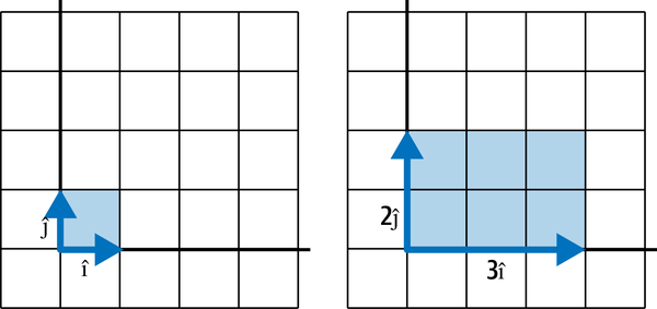
Figure 4-20. A determinant measures how a linear transformation scales an area

Note it increases in area by a factor of 6.0, and this factor is known as a determinant. Determinants describe how much a sampled area in a vector space changes in scale with linear transformations, and this can provide helpful information about the transformation.

Example 4-13 shows how to calculate this determinant in Python.

Example 4-13. Calculating a determinant

from numpy.linalg import det
from numpy import array

i_hat = array([3, 0])
j_hat = array([0, 2])

basis = array([i_hat, j_hat]).transpose()

determinant = det(basis)

print(determinant) # prints 6.0

Simple shears and rotations should not affect the determinant, as the area will not change. Figure 4-21 and Example 4-14 shows a simple shear and the determinant remains a factor 1.0, showing it is unchanged.

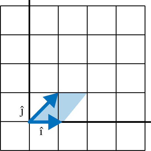
Figure 4-21. A simple shear does not change the determinant

Example 4-14. A determinant for a shear

from numpy.linalg import det
from numpy import array

i_hat = array([1, 0])
j_hat = array([1, 1])

basis = array([i_hat, j_hat]).transpose()

determinant = det(basis)

print(determinant) # prints 1.0

But scaling will increase or decrease the determinant, as that will increase/decrease the sampled area. When the orientation flips ($\widehat{i}$, $\widehat{j}$ swap clockwise positions), then the determinant will be negative. Figure 4-22 and Example 4-15 illustrate a determinant showing a transformation that not only scaled but also flipped the orientation of the vector space.

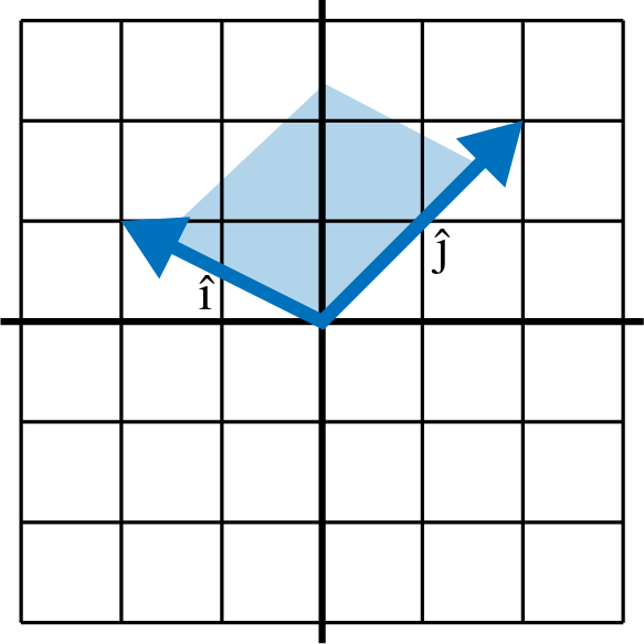
Figure 4-22. A determinant on a flipped space is negative

Example 4-15. A negative determinant

from numpy.linalg import det
from numpy import array

i_hat = array([-2, 1])
j_hat = array([1, 2])

basis = array([i_hat, j_hat]).transpose()

determinant = det(basis)

print(determinant) # prints -5.0

Because this determinant is negative, we quickly see that the orientation has flipped. But by far the most critical piece of information the determinant tells you is whether the transformation is linearly dependent. If you have a determinant of 0, that means all of the space has been squished into a lesser dimension.

In Figure 4-23 we see two linearly dependent transformations, where a 2D space is compressed into one dimension and a 3D space is compressed into two dimensions. The area and volume respectively in both cases are 0!

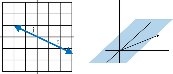
Figure 4-23. Linear dependence in 2D and 3D

Example 4-16 shows the code for the preceding 2D example squishing an entire 2D space into a single one-dimensional number line.

Example 4-16. A determinant of zero

from numpy.linalg import det
from numpy import array

i_hat = array([3, -1.5])
j_hat = array([-2, 1])

basis = array([i_hat, j_hat]).transpose()

determinant = det(basis)

print(determinant) # prints 0.0

So testing for a 0 determinant is highly helpful to determine if a transformation has linear dependence. When you encounter this you will likely find a difficult or unsolvable problem on your hands.

Special Types of Matrices

There are a few notable cases of matrices that we should cover.

Square Matrix

The square matrix is a matrix that has an equal number of rows and columns:

$$\left[\begin{array}{ccc}4& 2& 7\\ 5& 1& 9\\ 4& 0& 1\end{array}\right]$$

They are primarily used to represent linear transformations and are a requirement for many operations like eigendecomposition.

Identity Matrix

The identity matrix is a square matrix that has a diagonal of 1s while the other values are 0:

$$\left[\begin{array}{ccc}1& 0& 0\\ 0& 1& 0\\ 0& 0& 1\end{array}\right]$$

What’s the big deal with identity matrices? Well, when you have an identity matrix, you essentially have undone a transformation and found your starting basis vectors. This will play a big role in solving systems of equations in the next section.

Inverse Matrix

An inverse matrix is a matrix that undoes the transformation of another matrix. Let’s say I have matrix A:

$$A=\left[\begin{array}{ccc}4& 2& 4\\ 5& 3& 7\\ 9& 3& 6\end{array}\right]$$

The inverse of matrix A is called $A^{-1}$. We will learn how to calculate the inverse using Sympy or NumPy in the next section, but this is what the inverse of matrix A is:

$$A^{-1}=\left[\begin{array}{ccc}-\frac{1}{2}& 0& \frac{1}{3}\\ 5.5& -2& -\frac{4}{3}\\ -2& 1& \frac{1}{3}\end{array}\right]$$

When we perform matrix multiplication between $A^{-1}$ and A, we end up with an identity matrix. We will see this in action with NumPy and Sympy in the next section on systems of equations.

$$\left[\begin{array}{ccc}-\frac{1}{2}& 0& \frac{1}{3}\\ 5.5& -2& -\frac{4}{3}\\ -2& 1& \frac{1}{3}\end{array}\right]\left[\begin{array}{ccc}4& 2& 4\\ 5& 3& 7\\ 9& 3& 6\end{array}\right]=\left[\begin{array}{ccc}1& 0& 0\\ 0& 1& 0\\ 0& 0& 1\end{array}\right]$$

Diagonal Matrix

Similar to the identity matrix is the diagonal matrix, which has a diagonal of nonzero values while the rest of the values are 0. Diagonal matrices are desirable in certain computations because they represent simple scalars being applied to a vector space. It shows up in some linear algebra operations.

$$\left[\begin{array}{ccc}4& 0& 0\\ 0& 2& 0\\ 0& 0& 5\end{array}\right]$$

Triangular Matrix

Similar to the diagonal matrix is the triangular matrix, which has a diagonal of nonzero values in front of a triangle of values, while the rest of the values are 0.

$$\left[\begin{array}{ccc}4& 2& 9\\ 0& 1& 6\\ 0& 0& 5\end{array}\right]$$

Triangular matrices are desirable in many numerical analysis tasks, because they typically are easier to solve in systems of equations. They also show up in certain decomposition tasks like LU Decomposition.

Sparse Matrix

Occasionally, you will run into matrices that are mostly zeroes and have very few nonzero elements. These are called sparse matrices. From a pure mathematical standpoint, they are not terribly interesting. But from a computing standpoint, they provide opportunities to create efficiency. If a matrix has mostly 0s, a sparse matrix implementation will not waste space storing a bunch of 0s, and instead only keep track of the cells that are nonzero.

$$\text{sparse:}\left[\begin{array}{ccc}0& 0& 0\\ 0& 0& 2\\ 0& 0& 0\\ 0& 0& 0\end{array}\right]$$

When you have large matrices that are sparse, you might explicitly use a sparse function to create your matrix.

Systems of Equations and Inverse Matrices

One of the basic use cases for linear algebra is solving systems of equations. It is also a good application to learn about inverse matrices. Let’s say you are provided with the following equations and you need to solve for x, y, and z:

$$4x+2y+4z=44$$$$5x+3y+7z=56$$$$9x+3y+6z=72$$

You can try manually experimenting with different algebraic operations to isolate the three variables, but if you want a computer to solve it you will need to express this problem in terms of matrices as shown next. Extract the coefficients into matrix A, the values on the right side of the equation into matrix B, and the unknown variables into matrix X:

$$\begin{array}{c}\hfill A=\left[\begin{array}{ccc}4& 2& 4\\ 5& 3& 7\\ 9& 3& 6\end{array}\right]\\ \\ \\ \end{array}$$$$\begin{array}{c}\hfill B=\left[\begin{array}{c}44\\ 56\\ 72\end{array}\right]\\ \\ \\ \end{array}$$$$\begin{array}{c}\hfill X=\left[\begin{array}{c}x\\ y\\ z\end{array}\right]\end{array}$$

The function for a linear system of equations is AX = B. We need to transform matrix A with some other matrix X that will result in matrix B:

$$\begin{array}{c}\hfill AX=B\\ \\ \end{array}$$$$\begin{array}{c}\hfill \left[\begin{array}{ccc}4& 2& 4\\ 5& 3& 7\\ 9& 3& 6\end{array}\right]·\left[\begin{array}{c}x\\ y\\ z\end{array}\right]=\left[\begin{array}{c}44\\ 56\\ 72\end{array}\right]\end{array}$$

We need to “undo” A so we can isolate X and get the values for x, y, and z. The way you undo A is to take the inverse of A denoted by $A^{-1}$ and apply it to A via matrix multiplication. We can express this algebraically:

$$AX=B$$$$A^{-1}AX=A^{-1}B$$$$X=A^{-1}B$$

To calculate the inverse of matrix A, we probably use a computer rather than searching for solutions by hand using Gaussian elimination, which we will not venture into in this book. Here is the inverse of matrix A:

$$A^{-1}=\left[\begin{array}{ccc}-\frac{1}{2}& 0& \frac{1}{3}\\ 5.5& -2& \frac{4}{3}\\ -2& 1& \frac{1}{3}\end{array}\right]$$

Note when we matrix multiply $A^{-1}$ against A it will create an identity matrix, a matrix of all zeroes except for 1s in the diagonal. The identity matrix is the linear algebra equivalent of multiplying by 1, meaning it essentially has no effect and will effectively isolate values for x, y, and z:

$$\begin{array}{c}\hfill A^{-1}=\left[\begin{array}{ccc}-\frac{1}{2}& 0& \frac{1}{3}\\ 5.5& -2& \frac{4}{3}\\ -2& 1& \frac{1}{3}\end{array}\right]\\ \\ \end{array}$$$$\begin{array}{c}\hfill A=\left[\begin{array}{ccc}4& 2& 4\\ 5& 3& 7\\ 9& 3& 6\end{array}\right]\\ \end{array}$$$$\begin{array}{c}\hfill A^{-1}A=\left[\begin{array}{ccc}1& 0& 0\\ 0& 1& 0\\ 0& 0& 1\end{array}\right]\end{array}$$

To see this identity matrix in action in Python, you will want to use SymPy instead of NumPy. The floating point decimals in NumPy will not make the identity matrix as obvious, but doing it symbolically in Example 4-17 we will see a clean, symbolic output. Note that to do matrix multiplication in SymPy we use the asterisk * rather than @.

Example 4-17. Using SymPy to study the inverse and identity matrix

from sympy import *

# 4x + 2y + 4z = 44
# 5x + 3y + 7z = 56
# 9x + 3y + 6z = 72

A = Matrix([
    [4, 2, 4],
    [5, 3, 7],
    [9, 3, 6]
])

# dot product between A and its inverse
# will produce identity function
inverse = A.inv()
identity = inverse * A

# prints Matrix([[-1/2, 0, 1/3], [11/2, -2, -4/3], [-2, 1, 1/3]])
print("INVERSE: {}".format(inverse))

# prints Matrix([[1, 0, 0], [0, 1, 0], [0, 0, 1]])
print("IDENTITY: {}".format(identity))

In practice, the lack of floating point precision will not affect our answers too badly, so using NumPy should be fine to solve for x. Example 4-18 shows a solution with NumPy.

Example 4-18. Using NumPy to solve a system of equations

from numpy import array
from numpy.linalg import inv

# 4x + 2y + 4z = 44
# 5x + 3y + 7z = 56
# 9x + 3y + 6z = 72

A = array([
    [4, 2, 4],
    [5, 3, 7],
    [9, 3, 6]
])

B = array([
    44,
    56,
    72
])

X = inv(A).dot(B)

print(X) # [ 2. 34. -8.]

So x = 2, y = 34, and z = –8. Example 4-19 shows the full solution in SymPy as an alternative to NumPy.

Example 4-19. Using SymPy to solve a system of equations

from sympy import *

# 4x + 2y + 4z = 44
# 5x + 3y + 7z = 56
# 9x + 3y + 6z = 72

A = Matrix([
    [4, 2, 4],
    [5, 3, 7],
    [9, 3, 6]
])

B = Matrix([
    44,
    56,
    72
])

X = A.inv() * B

print(X) # Matrix([[2], [34], [-8]])

Here is the solution in mathematical notation:

$$\begin{array}{c}\hfill A^{-1}B=X\\ \\ \end{array}$$$$\begin{array}{c}\hfill \left[\begin{array}{ccc}-\frac{1}{2}& 0& \frac{1}{3}\\ 5.5& -2& \frac{4}{3}\\ -2& 1& \frac{1}{3}\end{array}\right]\left[\begin{array}{c}44\\ 56\\ 72\end{array}\right]=\left[\begin{array}{c}x\\ y\\ z\end{array}\right]\\ \\ \\ \end{array}$$$$\begin{array}{c}\hfill \left[\begin{array}{c}2\\ 34\\ -8\end{array}\right]=\left[\begin{array}{c}x\\ y\\ z\end{array}\right]\end{array}$$

Hopefully, this gave you an intuition for inverse matrices and how they can be used to solve a system of equations.

Systems of Equations in Linear Programming

This method of solving systems of equations is used for linear programming as well, where inequalities define constraints and an objective is minimized/maximized.

PatrickJMT has a lot of good videos on Linear Programming. We also cover it briefly in Appendix A.

In practicality, you should rarely find it necessary to calculate inverse matrices by hand and can have a computer do it for you. But if you have a need or are curious, you will want to learn about Gaussian elimination. PatrickJMT on YouTube has a number of videos demonstrating Gaussian elimination.

Eigenvectors and Eigenvalues

Matrix decomposition is breaking up a matrix into its basic components, much like factoring numbers (e.g., 10 can be factored to 2 × 5).

Matrix decomposition is helpful for tasks like finding inverse matrices and calculating determinants, as well as linear regression. There are many ways to decompose a matrix depending on your task. In Chapter 5 we will use a matrix decomposition technique, QR decomposition, to perform a linear regression.

But in this chapter let’s focus on a common method called eigendecomposition, which is often used for machine learning and principal component analysis. At this level we do not have the bandwidth to dive into each of these applications. For now, just know eigendecomposition is helpful for breaking up a matrix into components that are easier to work with in different machine learning tasks. Note also it only works on square matrices.

In eigendecomposition, there are two components: the eigenvalues denoted by lambda $\lambda$ and eigenvector by v shown in Figure 4-24.

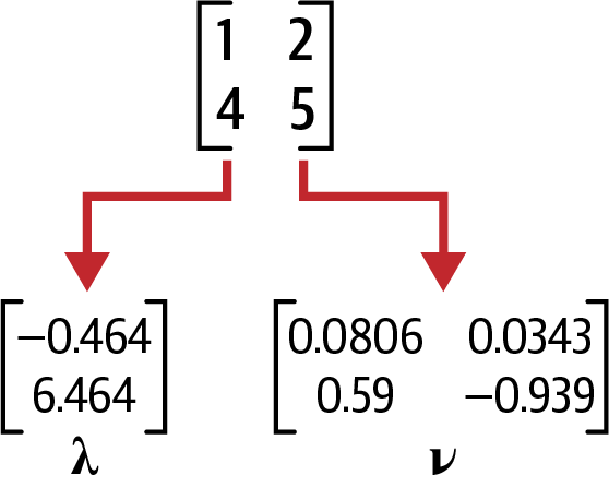
Figure 4-24. The eigenvector and eigenvalues

If we have a square matrix A, it has the following eigenvalue equation:

$Av=\lambda v$

If A is the original matrix, it is composed of eigenvector $v$ and eigenvalue $\lambda$. There is one eigenvector and eigenvalue for each dimension of the parent matrix, and not all matrices can be decomposed into an eigenvector and eigenvalue. Sometimes complex (imaginary) numbers will even result.

Example 4-20 is how we calculate eigenvectors and eigenvalues in NumPy for a given matrix $A$.

Example 4-20. Performing eigendecomposition in NumPy

from numpy import array, diag
from numpy.linalg import eig, inv

A = array([
    [1, 2],
    [4, 5]
])

eigenvals, eigenvecs = eig(A)

print("EIGENVALUES")
print(eigenvals)
print("\nEIGENVECTORS")
print(eigenvecs)

"""
EIGENVALUES
[-0.46410162  6.46410162]

EIGENVECTORS
[[-0.80689822 -0.34372377]
 [ 0.59069049 -0.9390708 ]]
"""

So how do we rebuild matrix A from the eigenvectors and eigenvalues? Recall this formula:

$Av=\lambda v$

We need to make a few tweaks to the formula to reconstruct A:

$A=Q\Lambda Q^{-1}$

In this new formula, $Q$ is the eigenvectors, $\Lambda$ is the eigenvalues in diagonal form, and $Q^{-1}$ is the inverse matrix of $Q$. Diagonal form means the vector is padded into a matrix of zeroes and occupies the diagonal line in a similar pattern to an identity matrix.

Example 4-21 brings the example full circle in Python, starting with decomposing the matrix and then recomposing it.

Example 4-21. Decomposing and recomposing a matrix in NumPy

from numpy import array, diag
from numpy.linalg import eig, inv

A = array([
    [1, 2],
    [4, 5]
])

eigenvals, eigenvecs = eig(A)

print("EIGENVALUES")
print(eigenvals)
print("\nEIGENVECTORS")
print(eigenvecs)

print("\nREBUILD MATRIX")
Q = eigenvecs
R = inv(Q)

L = diag(eigenvals)
B = Q @ L @ R

print(B)

"""
EIGENVALUES
[-0.46410162  6.46410162]

EIGENVECTORS
[[-0.80689822 -0.34372377]
 [ 0.59069049 -0.9390708 ]]

REBUILD MATRIX
[[1. 2.]
 [4. 5.]]
"""

As you can see, the matrix we rebuilt is the one we started with.

Conclusion

Linear algebra can be maddeningly abstract and it is full of mysteries and ideas to ponder. You may find the whole topic is one big rabbit hole, and you would be right! However, it is a good idea to continue being curious about it if you want to have a long, successful data science career. It is the foundation for statistical computing, machine learning, and other applied data science areas. Ultimately, it is the foundation for computer science in general. You can certainly get away with not knowing it for a while but you will encounter limitations in your understanding at some point.

You may wonder how these ideas are practical as they may feel theoretical. Do not worry; we will see some practical applications throughout this book. But the theory and geometric interpretations are important to have intuition when you work with data, and by understanding linear transformations visually you are prepared to take on more advanced concepts that may be thrown at you later in your pursuits.

If you want to learn more about linear programming, there is no better place than 3Blue1Brown’s YouTube playlist “Essence of Linear Algebra”. The linear algebra videos from PatrickJMT are helpful as well.

If you want to get more comfortable with NumPy, the O’Reilly book Python for Data Analysis (2nd edition) by Wes McKinney is a recommended read. It does not focus much on linear algebra, but it does provide practical instruction on using NumPy, Pandas, and Python on datasets.

Exercises

1. Vector $\overrightarrow{v}$ has a value of [1, 2] but then a transformation happens. $\widehat{i}$ lands at [2, 0] and $\widehat{j}$ lands at [0, 1.5]. Where does $\overrightarrow{v}$ land?

2. Vector $\overrightarrow{v}$ has a value of [1, 2] but then a transformation happens. $\widehat{i}$ lands at [-2, 1] and $\widehat{j}$ lands at [1, -2]. Where does $\overrightarrow{v}$ land?

3. A transformation $\widehat{i}$ lands at [1, 0] and $\widehat{j}$ lands at [2, 2]. What is the determinant of this transformation?

4. Can two or more linear transformations be done in single linear transformation? Why or why not?

5. Solve the system of equations for x, y, and z:

   $$3x+1y+0z==54$$$$2x+4y+1z=12$$$$3x+1y+8z=6$$

6. Is the following matrix linearly dependent? Why or why not?

   $$\left[\begin{array}{cc}2& 1\\ 6& 3\end{array}\right]$$

Answers are in Appendix B.