Chapter 4. Reductions in Spark
This chapter focuses on reduction transformations on RDDs in Spark. In particular, we’ll work with RDDs of (key, value) pairs, which are a common data abstraction required for many operations in Spark. Some initial ETL operations may be required to get your data into a (key, value) form, but with pair RDDs you may perform any desired aggregation over a set of values.
Spark supports several powerful reduction transformations and actions. The most important reduction transformations are:
-
reduceByKey() -
combineByKey() -
groupByKey() -
aggregateByKey()
All of the *ByKey() transformations accept a source
RDD[(K, V)] and create a target
RDD[(K, C)] (for some transformations,
such as reduceByKey(), V and C
are the same). The function of these transformations
is to reduce all the values of a given key
(for all unique keys), by finding, for example:
-
The average of all values
-
The sum and count of all values
-
The mode and median of all values
-
The standard deviation of all values
Reduction Transformation Selection
As with mapper transformations, it’s important to select the right tool for the job. For some reduction operations (such
as finding the median), the reducer needs access to all the values at
the same time. For others, such as finding the sum or count
of all values, it doesn’t. If you want to find
the median of values per key, then groupByKey()
will be a good choice, but this transformation
does not do well if a key has lots of values
(which might cause an OOM problem). On the
other hand, if you want to find the sum or count
of all values, then reduceByKey() might
be a good choice: it merges the values for
each key using an associative and commutative
reduce function.
This chapter will show you how to use the most important Spark reduction transformations, through simple working PySpark examples. We will focus on the transformations most commonly used in Spark applications. I’ll also discuss the general concept of reduction, and monoids as a design principle for efficient reduction algorithms. We’ll start by looking at how to create pair RDDs, which are required by Spark’s reduction transformations.
Creating Pair RDDs
Given a set of keys and their associated
values, a reduction transformation reduces the values of each
key using an algorithm (sum of value,
median of values, etc.). The reduction
transformations presented in this chapter
thus work on (key, value) pairs, which means that the RDD elements must conform to this format. There are several
ways to create pair RDDs in Spark. For example, you can also use
parallelize() on collections (such as lists of tuples and dictionaries), as shown here:
>>>key_value=[('A',2),('A',4),('B',5),('B',7)]>>>pair_rdd=spark.sparkContext.parallelize(key_value)>>>pair_rdd.collect()[('A',2),('A',4),('B',5),('B',7)]>>>pair_rdd.count()4>>>hashmap=pair_rdd.collectAsMap()>>>hashmap{'A':4,'B':7}

pair_rddhas two keys,{'A', 'B'}.
Next, suppose you have weather-related data and you
want to create pairs of (city_id, temperature). You can do this using the map() transformation.
Assume that your input has the following format:
<city_id><,><latitude><,><longitude><,><temperature>
First, define a function to create the desired (key, value) pairs:
defcreate_key_value(rec):tokens=rec.split(",")city_id=tokens[0]temperature=tokens[3]return(city_id,temperature)
The key is
city_idand the value istemperature.
Then use map() to create your pair RDD:
input_path=<your-temperature-data-path>rdd=spark.sparkContext.textFile(input_path)pair_rdd=rdd.map(create_key_value)# or you can write this using a lambda expression as:# pair_rdd = rdd.map(lambda rec: create_key_value(rec))
The are many other ways to create (key, value)
pair RDDs: reduceByKey(), for example, accepts a source RDD[(K, V)]
and produces a target RDD[(K, V)], and combineByKey() accepts a source RDD[(K, V)] and produces a target RDD[(K, C)].
Reduction Transformations
Typically, a reduction transformation reduces the data size from a large batch of values (such as list of numbers) to a smaller one. Examples of reductions include:
-
Finding the sum and average of all values
-
Finding the mean, mode, and median of all values
-
Calculating the mean and standard deviation of all values
-
Finding the
(min, max, count)of all values -
Finding the top 10 of all values
In a nutshell, a reduction transformation roughly corresponds to the fold operation (also called reduce, accumulate, or aggregate) in functional programming. The transformation is either applied to all data elements (such as when finding the sum of all elements) or to all elements per key (such as when finding the sum of all elements per key).
A simple addition reduction over a set
of numbers {47, 11, 42, 13} for a single
partition is illustrated in Figure 4-1.
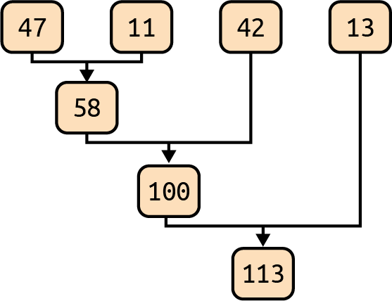
Figure 4-1. An addition reduction in a single partition
Figure 4-2 shows a reduction that sums the elements of two partitions.
The final reduced values for Partition-1
and Partition-2 are 21 and 18. Each
partition performs local reductions and
finally, the results from the two partitions are
reduced.
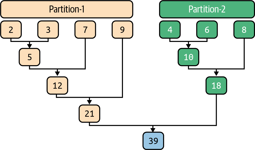
Figure 4-2. An addition reduction over two partitions
The reducer is a core concept in functional
programming, used to transform a set of objects
(such as numbers, strings, or lists) into
a single value (such as the sum of numbers or
concatenation of string objects). Spark and the
MapReduce paradigm use this concept
to aggregate a set of values into a single
value per key. Consider the following
(key, value) pairs, where the key is a
String and the value is a list of Integers:
(key1, [1, 2, 3])
(key2, [40, 50, 60, 70, 80])
(key3, [8])
The simplest reducer will be an addition function over a set of values per key. After we apply this function, the result will be:
(key1, 6)
(key2, 300)
(key3, 8)
Or you may reduce each (key, value)
to (key, pair) where the pair is
(sum-of-values, count-of-values):
(key1, (6, 3))
(key2, (300, 5))
(key3, (8, 1))
Reducers are designed to operate concurrently and independently, meaning that there is no synchronization between reducers. The more resources a Spark cluster has, the faster reductions can be done. In the worst possible case, if we have only one reducer, then reduction will work as a queue operation. In general, a cluster will offer many reducers (depending on resource availability) for the reduction transformation.
In MapReduce and distributed algorithms, reduction is a required operation in solving a problem. In the MapReduce programming paradigm,
the programmer defines a mapper and
a reducer with the following map()
and reduce() signatures (note that [] denotes an iterable):
map()-
(K1, V1) → [(K2, V2)] reduce()-
(K2, [V2]) → [(K3, V3)]
The map() function maps a
(key1, value1) pair into
a set of (key2, value2)
pairs. After all the map operations are
completed, the sort and shuffle is done automatically (this functionality is provided
by the MapReduce paradigm, not implemented by the programmer). The
MapReduce sort and shuffle phase is very similar
to Spark’s groupByKey()
transformation.
The reduce() function reduces a
(key2, [value2]) pair into
a set of (key3, value3)
pairs. The convention is used
to denote a list of objects (or
an iterable list of objects).
Therefore, we can say that a reduction
transformation takes a list of values
and reduces it to a tangible result
(such as the sum of values, average of
values, or your desired data
structure).
Spark’s Reductions
Spark provides a rich set of easy-to-use reduction transformations. As stated at the beginning of this chapter, our focus will be on reductions of pair RDDs. Therefore, we will assume that each RDD has a
set of keys and for each key (such as K) we
have a set of values:
{ (K, V1), (K, V2), ..., (K, Vn) }
Table 4-1 lists the reduction transformations available in Spark.
| Transformation | Description |
|---|---|
|
Aggregates the values of each key using the given combine functions and a neutral “zero value” |
|
Generic function to combine the elements for each key using a custom set of aggregation functions |
|
Counts the number of elements for each key, and returns the result to the master as a dictionary |
|
Merges the values for each key using an associative function and a neutral “zero value” |
|
Groups the values for each key in the RDD into a single sequence |
|
Merges the values for each key using an associative and commutative reduce function |
|
Returns a subset of this RDD sampled by key, using variable sampling rates for different keys as specified by fractions |
|
Sorts the RDD by key, so that each partition contains a sorted range of the elements in ascending order |
These transformation functions all act on (key, value) pairs represented by RDDs. In this chapter, we will look only at
reductions of data over a set of given
unique keys. For example, given the
following (key, value) pairs for the key K:
{ (K, V1), (K, V2), ..., (K, Vn) }
we are assuming that K has a list
of n (> 0) values:
[ V1, V2, ..., Vn ]
To keep it simple, the goal of reduction is to generate the following pair (or set of pairs):
(K, R)
where:
f(V1, V2, ..., Vn) -> R
The function f() is called a
reducer or reduction function.
Spark’s reduction transformations apply this function over a list of values to find the reduced value, R. Note that Spark does
not impose any ordering among the values
([V1, V2, ..., Vn]) to be reduced.
This chapter will include practical examples of solutions demonstrating the use of the most common of Spark’s reduction transformations: reduceByKey(), groupByKey(), aggregateByKey(), and combineByKey().
To get you started, let’s look at a very simple example of the groupByKey() transformation. As the example in Figure 4-3 shows, it works similarly to the SQL GROUP BY statement. In this example, we have four keys, {A, B, C, P}, and their associated values are grouped as a list of integers. The source RDD is an RDD[(String, Integer)], where each element is a pair of (String, Integer). The target RDD is an RDD[(String, [Integer])], where each element is a pair of (String, [Integer]); the value is an iterable list of integers.
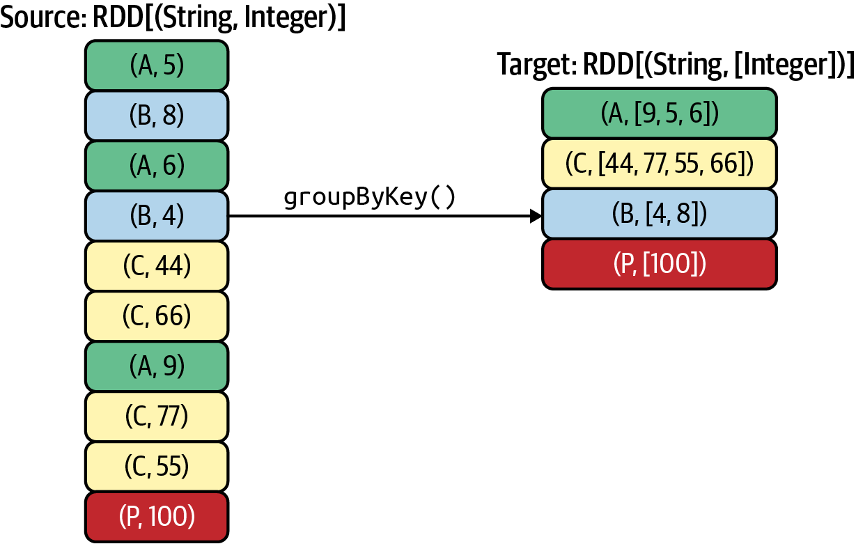
Figure 4-3. The groupByKey() transformation
Note
By default, Spark reductions do not sort the reduced values. For example, in Figure 4-3, the reduced value for key B could be [4, 8] or [8, 4]. If desired, you may sort the values before the final reduction. If your reduction algorithm requires sorting, you must sort the values explicitly.
Now that you have a general understanding of how reducers work, let’s move on to a practical example that demonstrates how different Spark reduction transformations can be used to solve a data problem.
Simple Warmup Example
Suppose we have a list of pairs (K, V),
where K (the key) is a String and V (the value) is an Integer:
[
 ('alex', 2), ('alex', 4), ('alex', 8),
 ('jane', 3), ('jane', 7),
 ('rafa', 1), ('rafa', 3), ('rafa', 5), ('rafa', 6),
 ('clint', 9)
]
In this example, we have four unique keys:
{ 'alex', 'jane', 'rafa', 'clint' }
Suppose we want to combine (sum) the values per key. The result of this reduction will be:
[
 ('alex', 14),
 ('jane', 10),
 ('rafa', 15),
 ('clint', 9)
]
where:
key: alex =>    14 = 2+4+8
key: jane =>    10 = 3+7
key: rafa =>    15 = 1+3+5+6
key: clint =>    9 (single value, no operation is done)
There are many ways to add these numbers to get the desired result. How did we arrive at these reduced (key, value) pairs? For this example, we could use any of the common Spark transformations. Aggregating or combining the values per key is a type of reduction—in the classic MapReduce paradigm, this is called a reduce by key (or simply reduce) function. The MapReduce framework calls the application’s (user-defined) reduce function once for each unique key. The function iterates through the values that are associated with that key and produces zero or more outputs as (key, value) pairs, solving the problem of combining the elements of each unique key into a single value. (Note that in some applications, the result might be more than a single value.)
Here I present four different solutions using
Spark’s transformations. For all solutions,
we will use the following Python data and
key_value_pairs RDD:
>>>data=[('alex',2),('alex',4),('alex',8),('jane',3),('jane',7),('rafa',1),('rafa',3),('rafa',5),('rafa',6),('clint',9)]>>>key_value_pairs=spark.SparkContext.parallelize(data)>>>key_value_pairs.collect()[('alex',2),('alex',4),('alex',8),('jane',3),('jane',7),('rafa',1),('rafa',3),('rafa',5),('rafa',6),('clint',9)]
datais a Python collection—a list of (key, value) pairs.
key_value_pairsis anRDD[(String, Integer)].
Solving with reduceByKey()
Summing the values for a given key is pretty
straightforward: add the first two values, then the next one, and
keep going. Spark’s reduceByKey() transformation merges the values for each key using an associative and commutative reduce function. Combiners (optimized mini-reducers) are used in all cluster nodes before merging the values per partition.
For the reduceByKey() transformation, the source RDD is an RDD[(K, V)] and the target RDD is an RDD[(K, V)]. Note that source and target data types of the
RDD values (V) are the same. This is a
limitation of reduceByKey(), which can be avoided by using
combineByKey() or aggregateByKey()).
We can apply the reduceByKey() transformation using a lambda expression (anonymous function):
# a is (an accumulated) value for key=K# b is a value for key=Ksum_per_key=key_value_pairs.reduceByKey(lambdaa,b:a+b)sum_per_key.collect()[('jane',10),('rafa',15),('alex',14),('clint',9)]
Alternatively, we can use a defined function, such as add:
fromoperatorimportaddsum_per_key=key_value_pairs.reduceByKey(add)sum_per_key.collect()[('jane',10),('rafa',15),('alex',14),('clint',9)]
Adding values per key by reduceByKey() is
an optimized solution, since aggregation happens at the partition level before the final aggregation
of all the partitions.
Solving with groupByKey()
We can also solve this problem by using the groupByKey()
transformation, but this solution will not perform as well because it involves moving lots of data to
the reducer nodes (you’ll learn more about why this is the case when we discuss the shuffle step later in this chapter).
With the reduceByKey() transformation, the source RDD is an RDD[(K, V)] and the target RDD is an RDD[(K, [V])]. Note that the source and target data types are not
the same: the value data type for the source RDD
is V, while for the target RDD it is [V] (an iterable/list of Vs).
The following example demonstrates the use of groupByKey() with a lambda expression to sum the values per key:
sum_per_key=key_value_pairs.grouByKey().mapValues(lambdavalues:sum(values))sum_per_key.collect()[('jane',10),('rafa',15),('alex',14),('clint',9)]
Group values per key (similar to SQL’s
GROUP BY). Now each key will have a set ofIntegervalues; for example, the three pairs{('alex', 2), ('alex', 4), ('alex', 8)}will be reduced to a single pair,('alex', [2, 4, 8]).Add values per key using Python’s
sum()function.
Solving with aggregateByKey()
In simplest form, the aggregateByKey()
transformation is defined as:
aggregateByKey(zero_value, seq_func, comb_func)

source RDD: RDD[(K, V)]
target RDD: RDD[(K, C))
It aggregates the values of each key from the source RDD into a target RDD, using the
given combine functions and a neutral
“zero value” (the initial value used for each partition). This function can return
a different result type (C) than the
type of the
values in the source RDD (V), though in this example both are Integer data types. Thus, we need one operation
for merging values within a single partition (merging values of type V into a value of type C) and one operation for merging values between partitions (merging values of type C from multiple partitions). To avoid unnecessary memory
allocation, both of these functions
are allowed to modify and return their
first argument instead of creating a
new C.
The following example demonstrates the use of the aggregateByKey()
transformation:
# zero_value -> C# seq_func: (C, V) -> C# comb_func: (C, C) -> C>>>sum_per_key=key_value_pairs.aggregateByKey(...0,...(lambdaC,V:C+V),...(lambdaC1,C2:C1+C2)...)>>>sum_per_key.collect()[('jane',10),('rafa',15),('alex',14),('clint',9)]
The
zero_valueapplied on each partition is0.seq_funcis used on a single partition.
comb_funcis used to combine the values of partitions.
Solving with combineByKey()
The combineByKey() transformation is the
most general and powerful of Spark’s reduction transformations. In its simplest form, it is defined
as:
combineByKey(create_combiner, merge_value, merge_combiners)

source RDD: RDD[(K, V)]
target RDD: RDD[(K, C))
Like aggregateByKey(), the combineByKey() transformation turns a source
RDD[(K, V)] into a target RDD[(K, C)]. Again, V and C
can be different data types (this is part of the power
of combineByKey()—for example, V can be a String or Integer, while C can be a list, tuple, or dictionary), but for this example
both are Integer data types.
The combineByKey() interface allows us
to customize the reduction and combining behavior as well as the data type. Thus, to use this transformation we have
to provide three functions:
create_combiner-
This function turns a single
Vinto aC(e.g., creating a one-element list). It is used within a single partition to initialize aC. merge_value-
This function merges a
Vinto aC(e.g., adding it to the end of a list). This is used within a single partition to aggregate values into aC. merge_combiners-
This function combines two
Cs into a singleC(e.g., merging the lists). This is used in merging values from two partitions.
Our solution with combineByKey() looks like this:
>>>sum_per_key=key_value_pairs.combineByKey(...(lambdav:v),...(lambdaC,v:C+v),...(lambdaC1,C2:C1+C2)...)>>>sum_per_key.collect()[('jane',10),('rafa',15),('alex',14),('clint',9)]
create_combinercreates the initial values in each partition.merge_valuemerges the values in a partition.merge_combinersmerges the values from the different partitions into the final result.
To give you a better idea of the power of the combineByKey()
transformation, let’s look at another example. Suppose we want to find the mean of values
per key. To solve this, we can create a combined
data type (C) as (sum, count), which will
hold the sums of values and their associated
counts:
# C = combined type as (sum, count)>>>sum_count_per_key=key_value_pairs.combineByKey(...(lambdav:(v,1)),...(lambdaC,v:(C[0]+v,C[1]+1),...(lambdaC1,C2:(C1[0]+C2[0],C1[1]+C2[1]))...)>>>mean_per_key=sum_count_per_key.mapValues(lambdaC:C[0]/C[1])
Given three partitions named {P1, P2, P3},
Figure 4-4 shows how to create a
combiner (data type C), how to merge a
value into a combiner, and finally how to
merge two combiners.
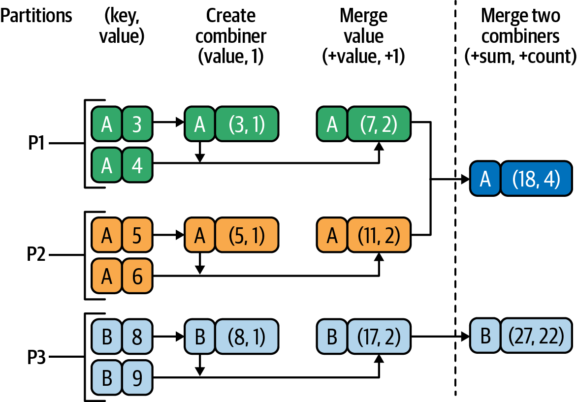
Figure 4-4. combineByKey() transformation example
Next, I will discuss the concept of monoids, which will help you to understand how combiners function in reduction transformations.
What Is a Monoid?
Monoids are a useful design principle for writing efficient MapReduce algorithms.1 If you don’t understand monoids, you might write reducer algorithms that do not produce semantically correct results. If your reducer is a monoid, then you can be sure that it will produce correct output in a distributed environment.
Since Spark’s reductions execute on a partition-by-partition basis (i.e., your reducer function is distributed rather than being a sequential function), to get the proper output you need to make sure that your reducer function is semantically correct. We’ll look at some examples of using monoids shortly, but first let’s examine the underlying mathematical concept.
In algebra, a monoid is an algebraic structure with a single associative binary operation and an identity element (also called a zero element).
For our purposes, we can informally define a monoid as M = (T, f, Zero), where:
-
Tis a data type. -
f()is a binary operation:f: (T, T) -> T. -
Zerois an instance ofT.
Note
Zero is an identity (neutral) element of
type T; this is not necessarily the number zero.
If a, b, c, and Zero are of type T, for the triple (T, f, Zero) to be a monoid the following properties must hold:
-
Binary operation
f: (T, T) -> T
-
Neutral element
for all a in T:

f(Zero, a) = a
f(a, Zero) = a
-
Associativity
for all a, b, c in T:

f(f(a, b), c) = f(a, f(b, c))
Not every binary operation
is a monoid. For example, the mean() function over a set of integers is not an associative function and therefore is not a monoid, as the following proof shows:
mean(10, mean(30, 50)) != mean(mean(10, 30), 50)

where

   mean(10, mean(30, 50))
      = mean (10, 40)
      = 25

   mean(mean(10, 30), 50)
      = mean (20, 50)
      = 35

   25 != 35
What does this mean? Given an
RDD[(String, Integer)], we might be tempted
to write the following transformation
to find an average per key:
# rdd: RDD[(String, Integer)]# WRONG REDUCTION to find average by keyavg_by_key=rdd.reduceByKey(lambdax,y:(x+y)/2)
But this will not produce the correct results, because the average of averages is not an average—in other words, the mean/average
function used here is not a monoid. Suppose
that this rdd has three elements:
{("A", 1), ("A", 2), ("A", 3)}; {("A", 1), ("A", 2)} are in
partition 1 and {("A", 3)}
is in partition 2. Using the preceding solution will result in aggregated values of ("A", 1.5) for partition 1 and ("A", 3.0) for partition 2. Combining the results for the two partitions will then give us a final average of (1.5 + 3.0) / 2 = 2.25, which is not the correct result (the average of the three values is 2.0). If your reducer is a monoid, it is guaranteed to behave properly and produce correct results.
Monoid and Non-Monoid Examples
To help you understand and recognize monoids, let’s look at some monoid and non-monoid examples. The following are examples of monoids:
-
Integers with addition:
((a + b ) + c) = (a + (b + c))
0 + n = n
n + 0 = n
The zero element for addition is the number 0.
-
Integers with multiplication:
((a * b) * c) = (a * (b * c))
1 * n = n
n * 1 = n
The zero element for multiplication is the number 1.
-
Strings with concatenation:
(a + (b + c)) = ((a + b) + c)
"" + s = s
s + "" = s
The zero element for concatenation is an empty string of size 0.
-
Lists with concatenation:
List(a, b) + List(c, d) = List(a,b,c,d)
-
Sets with their union:
Set(1,2,3) + Set(2,4,5)
   = Set(1,2,3,2,4,5)
   = Set(1,2,3,4,5)

S + {} = S
{} + S = S
The zero element is an empty set {}.
And here are some non-monoid examples:
-
Integers with mean function:
mean(mean(a,b),c) != mean(a, mean(b,c))
-
Integers with subtraction:
((a - b) -c) != (a - (b - c))
-
Integers with division:
((a / b) / c) != (a / (b / c))
-
Integers with mode function:
mode(mode(a, b), c) != mode(a, mode(b, c))
-
Integers with median function:
median(median(a, b), c) != median(a, median(b, c))
In some cases, it is possible to convert a non-monoid into a monoid. For example, with a simple change to our data structures we can find the correct mean of a set of numbers. However, there is no algorithm to convert a non-monoid structure to a monoid automatically.
Writing distributed algorithms in Spark is much different from writing sequential algorithms on a single server, because the algorithms operate in parallel on partitioned data. Therefore, when writing a reducer, you need to make sure that your reduction function is a monoid. Now that you understand this important concept, let’s move on to some practical examples.
The Movie Problem
The goal of this first example is to present a basic problem and then provide solutions using different Spark reduction transformations by means of PySpark. For all reduction transformations, I have carefully selected the data types such that they form a monoid.
The movie problem can be stated as follows: given a
set of users, movies, and ratings, (in the range 1 to 5), we want to find the average rating of all
movies by a user. So, if the user with userID=100) has rated four movies:
(100, "Lion King", 4.0)
(100, "Crash", 3.0)
(100, "Dead Man Walking", 3.5)
(100, "The Godfather", 4.5)
we want to generate the following output:
(100, 3.75)
where:
3.75 = mean(4.0, 3.0, 3.5, 4.5)
     = (4.0 + 3.0 + 3.5 + 4.5) / 4
     = 15.0 / 4
For this example, note that the reduceByKey()
transformation over a set of ratings will not
always produce the correct output, since the average (or mean) is not an algebraic monoid over a set of float/integer numbers. In other words, as discussed in the previous section, the mean of means is not equal to the mean of all input numbers.
Here is a simple proof. Suppose we want to find the mean of six values (the numbers 1–6), stored in a single partition. We can do this with the mean() function as follows:
mean(1, 2, 3, 4, 5, 6)
   = (1 + 2 + 3 + 4 + 5 + 6) / 6
   = 21 / 6
   = 3.5 [correct result]
Now, let’s make mean() function as a distributed
function. Suppose the values are stored on three partitions:
Partition-1: (1, 2, 3)
Partition-2: (4, 5)
Partition-3: (6)
First, we compute the mean of each partition:
mean(1, 2, 3, 4, 5, 6)
  =  mean (
           mean(Partition-1),
           mean(Partition-2),
           mean(Partition-3)
          )

mean(Partition-1)
  = mean(1, 2, 3)
  = mean( mean(1,2), 3)
  = mean( (1+2)/2, 3)
  = mean(1.5, 3)
  = (1.5+3)/2
  = 2.25

mean(Partition-2)
  = mean(4,5)
  = (4+5)/2
  = 4.5

mean(Partition-3)
  = mean(6)
  = 6
Then we find the mean of these values. Once all partitions are processed, therefore, we get:
mean(1, 2, 3, 4, 5, 6)
  =  mean (
           mean(Partition-1),
           mean(Partition-2),
           mean(Partition-3)
          )
  = mean(2.25, 4.5, 6)
  = mean(mean(2.25, 4.5), 6)
  = mean((2.25 + 4.5)/2, 6)
  = mean(3.375, 6)
  = (3.375 + 6)/2
  = 9.375 / 2
  = 4.6875  [incorrect result]
To avoid this problem, we can
use a monoid data structure (which supports
associativity and commutativity) such as a
pair of (sum, count), where sum is the total
sum of all numbers we have seen so far (per partition) and count is the
number of ratings we have seen so far. If we define our mean() function as:
mean(pair(sum, count)) = sum / count
we get:
mean(1,2,3,4,5,6)
  = mean(mean(1,2,3), mean(4,5), mean(6))
  = mean(pair(1+2+3, 1+1+1), pair(4+5, 1+1), pair(6,1))
  = mean(pair(6, 3), pair(9, 2), pair(6,1))
  = mean(mean(pair(6, 3), pair(9, 2)), pair(6,1))
  = mean(pair(6+9, 3+2), pair(6,1))
  = mean(pair(15, 5), pair(6,1))
  = mean(pair(15+6, 5+1))
  = mean(pair(21, 6))
  = 21 / 6 = 3.5 [correct result]
As this example shows, by using a monoid we can achieve associativity.
Therefore, you may apply the reduceByKey() transformation when your function f() is commutative and associative:
# a = (sum1, count1)# b = (sum2, count2)# f(a, b) = a + b# = (sum1+sum2, count1+count2)#reduceByKey(lambdaa,b:f(a,b))
For example, the addition
(+) operation is commutative and associative,
but the mean/average function does not satisfy
these properties.
Note
As we saw in Chapter 1, a commutative function ensures that the result is independent of the order of elements in the RDD being aggregated:
f(A, B) = f(B, A)
An associative function ensures that the order in which elements are grouped during the aggregation does not affect the final result:
f(f(A, B), C) = f(A, f(B, C))
Input Dataset to Analyze
The sample data we’ll use for this problem is a dataset from MovieLens. For simplicity, I will assume that you have downloaded and unzipped the files into a /tmp/movielens/ directory. Note that there is no requirement to put the files at the suggested location; you may place your files in your preferred directory and update your input paths accordingly.
Tip
The full MovieLens dataset (ml-latest.zip) is 265 MB. If you want to use a smaller dataset to run, test, and debug the programs listed here, you can instead download the small MovieLens dataset, a 1 MB file consisting of 100,000 ratings and 3,600 tag applications applied to 9,000 movies by 600 users.
All ratings are contained in the file ratings.csv. Each line of this file after the header row represents one rating of one movie by one user, and has the following format:
<userId><,><movieId><,><rating><,><timestamp>
In this file:
-
The lines are ordered first by
userId, then, for each user, bymovieId. -
Ratings are made on a 5-star scale, with half-star increments (0.5 stars to 5.0 stars).
-
Timestamps represent seconds since midnight Coordinated Universal Time (UTC) of January 1, 1970 (this field is ignored in our analysis).
After unzipping the downloaded file, you should have the following files:
$ ls -l /tmp/movielens/
       8,305  README.txt
     725,770  links.csv
   1,729,811  movies.csv
 620,204,630  ratings.csv
  21,094,823  tags.csv
First, check the number of records (the number of records you see might be different based on when you downloaded the file):
$ wc -l /tmp/movielens/ratings.csv
22,884,378 /tmp/movielens/ratings.csv
Next, take a look at the first few records:
$ head -6 /tmp/movielens/ratings.csv
userId,movieId,rating,timestamp
1,169,2.5,1204927694
1,2471,3.0,1204927438
1,48516,5.0,1204927435
2,2571,3.5,1436165433
2,109487,4.0,1436165496
Since we are using RDDs, we do not need the metadata associated with the data. Therefore, we can remove the first line (the header line) from the ratings.csv file:
$ tail -n +2 ratings.csv > ratings.csv.no.header
$ wc -l ratings.csv ratings.csv.no.header
22,884,378 ratings.csv
22,884,377 ratings.csv.no.header
Now that we’ve acquired our sample data, we can work through a few solutions to this problem. The first solution will use aggregateByKey(), but before we get to that I’ll present the logic behind this transformation.
The aggregateByKey() Transformation
Spark’s aggregateByKey() transformation initializes each key on each partition with the zero value, which is an initial combined data type (C); this is a neutral value, typically (0, 0) if the combined data type is (sum, count). This zero value is
merged with the first value in the partition to create a new C, which is then merged with the second value. This process
continues until we’ve merged all the values for that key. Finally, if the same key exists in multiple partitions,
these values are combined together to produce the final C.
Figures 4-5 and 4-6 show how
aggregateByKey() works with different
zero values. The zero value is applied
per key, per partition. This means that
if a key X is in N partitions,
the zero value is applied N times
(each of these N partitions will be
initialized to the zero value for key X). Therefore, it’s important to select this value carefully.
Figure 4-5 demonstrates how aggregateByKey()
works with zero-value=(0, 0).

Figure 4-5. aggregateByKey() with zero-value=(0, 0)
Typically, you would use (0, 0) but Figure 4-6 demonstrates how the same transformation works with a zero value of (10, 20).
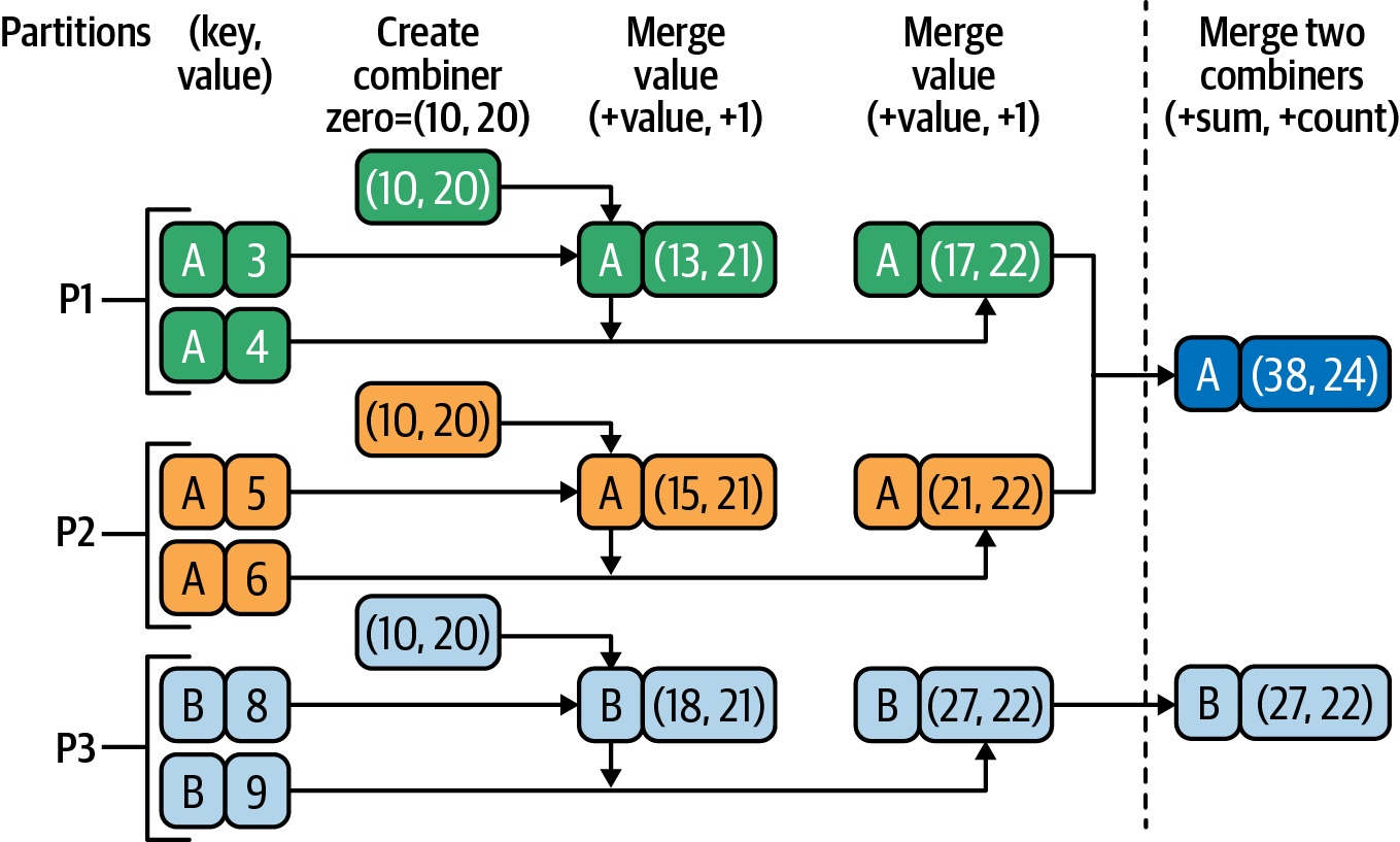
Figure 4-6. aggregateByKey() with zero-value=(10, 20)
First Solution Using aggregateByKey()
To find the average rating for each user, the first step is to map each record into (key, value) pairs of the form:
(userID-as-key, rating-as-value)
The simplest way to add up values
per key is to use the reduceByKey()
transformation, but we can’t use reduceByKey()
to find the average rating per user because, as we’ve seen,
the mean/average function is not a
monoid over a set of ratings (as
float numbers). To make this a monoid
operation, we use a pair data structure
(a tuple of two elements) to hold a pair
of values, (sum, count), where sum is
the aggregated sum of ratings and count
is the number of ratings we have added
(summed) so far, and we use the aggregateByKey() transformation.
Let’s prove that the pair structure
(sum, count) with an addition
operator over a set of numbers is
a monoid.
If we use (0.0, 0) as our zero element, it is neutral:
f(A, Zero) = A
f(Zero, A) = A

A = (sum, count)

f(A, Zero)
  = (sum+0.0, count+0)
  = (sum, count)
  = A

f(Zero, A)
  = (0.0+sum, 0+count)
  = (sum, count)
  = A
The operation is commutative (that is, the result is independent of the order of the elements in the RDD being aggregated):
f(A, B) = f(B, A)

A = (sum1, count1)
B = (sum2, count2)

f(A, B)
  = (sum1+sum2, count1+count2)
  = (sum2+sum1, count2+count1)
  = f(B, A)
It is also associative (the order in which elements are aggregated does not affect the final result):
f(f(A, B), C) = f(A, f(B, C))

A = (sum1, count1)
B = (sum2, count2)
C = (sum3, count3)

f(f(A, B), C)
  = f((sum1+sum2, count1+count2), (sum3, count3))
  = (sum1+sum2+sum3, count1+count2+count3)
  = (sum1+(sum2+sum3), count1+(count2+count3))
  = f(A, f(B, C))
To make things simple, we’ll define a very
basic Python function, create_pair(),
which accepts a record of movie rating
data and returns a pair of (userID, rating):
# Define a function that accepts a CSV record# and returns a pair of (userID, rating)# Parameters: rating_record (as CSV String)# rating_record = "userID,movieID,rating,timestamp"defcreate_pair(rating_record):tokens=rating_record.split(",")userID=tokens[0]rating=float(tokens[2])return(userID,rating)#end-def
Next, we test the function:
key_value_1=create_pair("3,2394,4.0,920586920")key_value_1('3',4.0)key_value_2=create_pair("1,169,2.5,1204927694")key_value_2('1',2.5)
Here is a PySpark solution using aggregateByKey() and our create_pair() function.
The combined type (C) to denote values for the
aggregateByKey() operation is a pair of (sum-of-ratings,
count-of-ratings).
# spark: an instance of SparkSessionratings_path="/tmp/movielens/ratings.csv.no.header"rdd=spark.sparkContext.textFile(ratings_path)# load user-defined Python functionratings=rdd.map(lambdarec:create_pair(rec))ratings.count()## C = (C[0], C[1]) = (sum-of-ratings, count-of-ratings)# zero_value -> C = (0.0, 0)# seq_func: (C, V) -> C# comb_func: (C, C) -> Csum_count=ratings.aggregateByKey((0.0,0),(lambdaC,V:(C[0]+V,C[1]+1)),(lambdaC1,C2:(C1[0]+C2[0],C1[1]+C2[1])))
The source RDD,
ratings, is anRDD[(String, Float)]where the key is auserIDand the value is arating.The target RDD,
sum_count, is anRDD[(String, (Float, Integer))]where the key is auserIDand the value is a pair(sum-of-ratings, count-of-ratings).Cis initialized to this value in each partition.
This is used to combine values within a single partition.

This is used to combine the results from different partitions.
Let’s break down what’s happening here. First, we the aggregateByKey() function and create a result set “template” with the initial values. We’re starting the data out as (0.0, 0), so the initial sum of ratings is 0.0 and the initial count of records is 0. For each row of data, we’re going to do some adding. C is the new template, so C[0] is referring to our “sum” element (sum-of-ratings), while C[1] is the “count” element (count-of-ratings). Finally, we combine the values from the different partitions. To do this, we simply add the C1 values to the C2 values based on the template we made.
The data in the sum_count RDD will end up
looking like the following:
sum_count=[(userID,(sum-of-ratings,count-of-ratings)),...]=RDD[(String,(Float,Integer))][(100,(40.0,10)),(200,(51.0,13)),(300,(340.0,90)),...]
This tells us that user 100 has rated 10 movies and the sum of all their ratings was 40.0; user 200 has rated 13 movies and the sum of their ratings was 51.0
Now, to get the actual average rating per user, we need to
use the mapValues() transformation and divide
the first entry (sum-of-ratings) by the second entry (count-of-ratings):
# x = (sum-of-ratings, count-of-ratings)# x[0] = sum-of-ratings# x[1] = count-of-ratings# avg = sum-of-ratings / count-of-ratingsaverage_rating=sum_count.mapValues(lambdax:(x[0]/x[1]))
average_ratingis anRDD[(String, Float)]where the key is auserIDand the value is anaverage-rating.
The contents of this RDD are as follows, giving us the result we’re looking for:
average_rating
[
  (100, 4.00),
  (200, 3.92),
  (300, 3.77),
  ...
]
Second Solution Using aggregateByKey()
Here, I’ll present another solution using the aggregateByKey() transformation. Note that to save space,
I have trimmed the output generated by the PySpark shell.
The first step is to read the data and create (key, value) pairs,
where the key is a userID and the value is a rating:
# ./bin/pysparkSparkSessionavailableas'spark'.>>># create_pair() returns a pair (userID, rating)>>># rating_record = "userID,movieID,rating,timestamp">>>defcreate_pair(rating_record):...tokens=rating_record.split(",")...return(tokens[0],float(tokens[2]))...>>>key_value_test=create_pair("3,2394,4.0,920586920")>>>key_value_test('3',4.0)>>>ratings_path="/tmp/movielens/ratings.csv.no.header">>>rdd=spark.sparkContext.textFile(ratings_path)>>>rdd.count()22884377>>>ratings=rdd.map(lambdarec:create_pair(rec))>>>ratings.count()22884377>>>ratings.take(3)[(u'1',2.5),(u'1',3.0),(u'1',5.0)]
Once we’ve created the (key, value) pairs, we can
apply the aggregateByKey() transformation to sum
up the ratings. The initial value of (0.0, 0)
is used for each partition, where 0.0 is the sum of
the ratings and 0 is the number of ratings:
>>># C is a combined data structure, (sum, count)>>>sum_count=ratings.aggregateByKey(...(0.0,0),...(lambdaC,V:(C[0]+V,C[1]+1)),...(lambdaC1,C2:(C1[0]+C2[0],C1[1]+C2[1])))>>>sum_count.count()247753>>>sum_count.take(3)[(u'145757',(148.0,50)),(u'244330',(36.0,17)),(u'180162',(1882.0,489))]
The target RDD is an
RDD[(String, (Float, Integer))].Cis initialized to(0.0, 0)in each partition.This lambda expression adds a single value of
VtoC(used in a single partition).This lambda expression combines the values across partitions (adds two
Cs to create a singleC).
We could use Python functions instead of lambda expressions. To do this, we would need to write the following functions:
# C = (sum, count)# V is a single value of type Floatdefseq_func(C,V):return(C[0]+V,C[1]+1)#end-def# C1 = (sum1, count1)# C2 = (sum2, count2)defcomb_func(C1,C2):return(C1[0]+C2[0],C1[1]+C2[1])#end-def
Now, we can compute sum_count
using the defined functions:
sum_count=ratings.aggregateByKey((0.0,0),seq_func,comb_func)
The previous step created RDD elements of the following type:
(userID, (sum-of-ratings, number-of-ratings))
Next, we do the final calculation to find the average rating per user:
>>># x refers to a pair of (sum-of-ratings, number-of-ratings)>>># where>>># x[0] denotes sum-of-ratings>>># x[1] denotes number-of-ratings>>>>>>average_rating=sum_count.mapValues(lambdax:(x[0]/x[1]))>>>average_rating.count()247753>>>average_rating.take(3)[(u'145757',2.96),(u'244330',2.1176470588235294),(u'180162',3.8486707566462166)]
Next, I’ll present a solution to the movies
problem using groupByKey().
Complete PySpark Solution Using groupByKey()
For a given set of (K, V) pairs,
groupByKey() has the following signature:
groupByKey(numPartitions=None,partitionFunc=<functionportable_hash>)groupByKey:RDD[(K,V)]-->RDD[(K,[V])]
If the source RDD is an RDD[(K, V)], the groupByKey() transformation
groups the values for each key (K)
in the RDD into a single sequence as a list/iterable of Vs. It then hash-partitions
the resulting RDD with the existing
partitioner/parallelism level. The
ordering of elements within each group
is not guaranteed, and may even differ
each time the resulting RDD is evaluated.
Tip
You can customize both the
number of partitions (numPartitions)
and partitioning function (partitionFunc).
Here, I present a complete solution using
the groupByKey() transformation.
The first step is to read the data and create (key, value) pairs,
where the key is a userID and the value is a rating:
>>># spark: SparkSession>>>defcreate_pair(rating_record):...tokens=rating_record.split(",")...return(tokens[0],float(tokens[2]))...>>>key_value_test=create_pair("3,2394,4.0,920586920")>>>key_value_test('3',4.0)>>>ratings_path="/tmp/movielens/ratings.csv.no.header">>>rdd=spark.sparkContext.textFile(ratings_path)>>>rdd.count()22884377>>>ratings=rdd.map(lambdarec:create_pair(rec))>>>ratings.count()22884377>>>ratings.take(3)[(u'1',2.5),(u'1',3.0),(u'1',5.0)]
ratingsis anRDD[(String, Float)]
Once we’ve created the (key, value) pairs, we
can apply the groupByKey() transformation
to group all ratings for a user. This step creates
(userID, [R1, ..., Rn]) pairs,
where R1, …, Rn are all of the
ratings for a unique userID.
As you will notice, the groupByKey()
transformation works exactly like SQL’s GROUP BY. It groups values of the same key as an iterable of values:
>>>ratings_grouped=ratings.groupByKey()>>>ratings_grouped.count()247753>>>ratings_grouped.take(3)[(u'145757',<ResultIterableobjectat0x111e42e50>),(u'244330',<ResultIterableobjectat0x111e42dd0>),(u'180162',<ResultIterableobjectat0x111e42e10>)]>>>ratings_grouped.mapValues(lambdax:list(x)).take(3)[(u'145757',[2.0,3.5,...,3.5,1.0]),(u'244330',[3.5,1.5,...,4.0,2.0]),(u'180162',[5.0,4.0,...,4.0,5.0])]
ratings_groupedis anRDD[(String, [Float])]where the key is auserIDand the value is a list ofratings.The full name of
ResultIterableispyspark.resultiterable.ResultIterable.For debugging, convert the
ResultIterableobject to a list ofIntegers.
To find the average rating per user, we sum up
all the ratings for each userID and then calculate the averages:
>>># x refers to all ratings for a user as [R1, ..., Rn]>>># x: ResultIterable object>>>average_rating=ratings_grouped.mapValues(lambdax:sum(x)/len(x))>>>average_rating.count()247753>>>average_rating.take(3)[(u'145757',2.96),(u'244330',2.12),(u'180162',3.85)]
Complete PySpark Solution Using reduceByKey()
In its simplest form, reduceByKey() has the following signature
(the source and target data types, V, must
be the same):
reduceByKey(func, numPartitions=None, partitionFunc)
reduceByKey: RDD[(K, V)] --> RDD[(K, V)]
reduceByKey() transformation merges
the values for each key using an
associative and commutative reduce
function. This will also perform the
merging locally on
each mapper before
sending the results to a reducer, similarly
to a combiner in
MapReduce. The output
will be partitioned with numPartitions
partitions, or the default parallelism
level if numPartitions is not specified.
The default partitioner is HashPartitioner.
Since we want to find the average rating
for all movies rated by a user, and we
know that the mean of means is not a mean (the mean
function is not a monoid), we need to add up all the ratings for each user and
keep track of the number of movies they’ve rated. Then, (sum_of_ratings, number_of_ratings) is a monoid over an addition function, but
at the end we need to perform one more mapValues()
transformation to find the actual average
rating by dividing sum_of_ratings by number_of_ratings. The complete solution
using reduceByKey() is given here.
Note that reduceByKey() is more efficient
and scalable than a groupByKey()
transformation, since merging and combining
are done locally before sending data
for the final reduction.
Step 1: Read data and create pairs
The first step is to read the data and create (key, value)
pairs, where the key is a userID and the value is
a pair of (rating, 1). To use reduceByKey()
for finding averages, we need to find the
(sum_of_ratings, number_of_ratings). We start by reading the input data and creating an RDD[String]:
>>># spark: SparkSession>>>ratings_path="/tmp/movielens/ratings.csv.no.header">>># rdd: RDD[String]>>>rdd=spark.sparkContext.textFile(ratings_path)>>>rdd.take(3)[u'1,169,2.5,1204927694',u'1,2471,3.0,1204927438',u'1,48516,5.0,1204927435']
Then we transform the RDD[String] into an RDD[(String, (Float, Integer))]:
>>>defcreate_combined_pair(rating_record):...tokens=rating_record.split(",")...userID=tokens[0]...rating=float(tokens[2])...return(userID,(rating,1))...>>># ratings: RDD[(String, (Float, Integer))]>>>ratings=rdd.map(lambdarec:create_combined_pair(rec))>>>ratings.count()22884377>>>ratings.take(3)[(u'1',(2.5,1)),(u'1',(3.0,1)),(u'1',(5.0,1))]
Create the pair RDD.
Step 2: Use reduceByKey() to sum up ratings
Once we’ve created the (userID, (rating, 1)) pairs we can apply the reduceByKey() transformation
to sum up all the ratings and the number of ratings for a given user. The
output of this step will be tuples of
(userID, (sum_of_ratings,
number_of_ratings)):
>>># x refers to (rating1, frequency1)>>># y refers to (rating2, frequency2)>>># x = (x[0] = rating1, x[1] = frequency1)>>># y = (y[0] = rating2, y[1] = frequency2)>>># x + y = (rating1+rating2, frequency1+frequency2)>>># ratings is the source RDD>>>sum_and_count=ratings.reduceByKey(lambdax,y:(x[0]+y[0],x[1]+y[1]))>>>sum_and_count.count()247753>>>sum_and_count.take(3)[(u'145757',(148.0,50)),(u'244330',(36.0,17)),(u'180162',(1882.0,489))]
The source RDD (
ratings) is anRDD[(String, (Float, Integer))].The target RDD (
sum_and_count) is anRDD[(String, (Float, Integer))]. Notice that the data types for the source and target are the same.
Step 3: Find average rating
Divide sum_of_ratings by number_of_ratings to find the average rating per user:
>>># x refers to (sum_of_ratings, number_of_ratings)>>># x = (x[0] = sum_of_ratings, x[1] = number_of_ratings)>>># avg = sum_of_ratings / number_of_ratings = x[0] / x[1]>>>avgRating=sum_and_count.mapValues(lambdax:x[0]/x[1])>>>avgRating.take(3)[(u'145757',2.96),(u'244330',2.1176470588235294),(u'180162',3.8486707566462166)]
Complete PySpark Solution Using combineByKey()
combineByKey() is a more general and extended
version of reduceByKey() where the result type
can be different than the type of the values being aggregated.
This is a limitation of reduceByKey(); it means that, given the
following:
# let rdd represent (key, value) pairs# where value is of type Trdd2=rdd.reduceByKey(lambdax,y:func(x,y))
func(x,y) must create a value of type T.
The combineByKey() transformation
is an optimization that aggregates
values for a given key before sending aggregated partition values to
the designated reducer. This aggregation is performed in each partition, and then the values from all the partitions are merged into a single
value. Thus, like with reduceByKey(), each partition outputs at most one value for each key to send over the network, which speeds up the shuffle step. However, unlike with reduceByKey(), the type of the combined
(result) value does not have to match the
type of the original value.
For a given set of (K, V) pairs, combineByKey()
has the following signature (this transformation
has many different versions; this is the simplest
form):
combineByKey(create_combiner, merge_value, merge_combiners)
combineByKey : RDD[(K, V)] --> RDD[(K, C)]

V and C can be different data types.
This is a generic function to combine
the elements for each key using a custom
set of aggregation functions. It converts
an RDD[(K, V)] into a result of type
RDD[(K, C)], where C is a combined type.
It can be a simple data type such as Integer or String, or it can be a composite
data structure such as a (key, value) pair, a triplet (x, y, z), or whatever else you desire. This flexibility, makes combineByKey()
a very powerful reducer.
As discussed earlier in this chapter, given a source RDD RDD[(K, V)], we
have to provide three basic functions:
create_combiner: (V) -> C
merge_value: (C, V) -> C
merge_combiners: (C, C) -> C
To avoid memory allocation, both merge_value
and merge_combiners are allowed to modify
and return their first argument instead of
creating a new C (this avoids creating
new objects, which can be costly if you have
a lot of data).
In addition, users can control (by providing
additional parameters) the partitioning of
the output RDD, the serializer that is used
for the shuffle, and whether to perform map-side
aggregation (i.e., if a mapper can produce multiple
items with the same key). The combineByKey()
transformation thus provides quite a bit of flexibility, but it is a little more complex to use than some of the other reduction transformations.
Let’s see how we can use combineByKey() to solve the movie problem.
Step 1: Read data and create pairs
As in the previous solutions, the first step is to read the data and create (key, value) pairs
where the key is a userID and the value is a rating:
>>># spark: SparkSession>>># create and return a pair of (userID, rating)>>>defcreate_pair(rating_record):...tokens=rating_record.split(",")...return(tokens[0],float(tokens[2]))...>>>key_value_test=create_pair("3,2394,4.0,920586920")>>>key_value_test('3',4.0)>>>ratings_path="/tmp/movielens/ratings.csv.no.header">>>rdd=spark.sparkContext.textFile(ratings_path)>>>rdd.count()22884377>>>ratings=rdd.map(lambdarec:create_pair(rec))>>>ratings.count()22884377>>>ratings.take(3)[(u'1',2.5),(u'1',3.0),(u'1',5.0)]
rddis anRDD[String].ratingsis anRDD[(String, Float)].
Step 2: Use combineByKey() to sum up ratings
Once we’ve created the (userID, rating) pairs , we can apply the combineByKey()
transformation to sum up all the ratings and the number of ratings for each user. The
output of this step will be (userID, (sum_of_ratings, number_of_ratings)) pairs:
>>># v is a rating from (userID, rating)>>># C represents (sum_of_ratings, number_of_ratings)>>># C[0] denotes sum_of_ratings>>># C[1] denotes number_of_ratings>>># ratings: source RDD>>>sum_count=ratings.combineByKey((lambdav:(v,1)),(lambdaC,v:(C[0]+v,C[1]+1)),(lambdaC1,C2:(C1[0]+C2[0],C1[1]+C2[1])))>>>sum_count.count()247753>>>sum_count.take(3)[(u'145757',(148.0,50)),(u'244330',(36.0,17)),(u'180162',(1882.0,489))]
The source RDD is an
RDD[(String, Float)].The target RDD is an
RDD[(String, (Float, Integer))].This turns a
V(a single value) into aCas(V, 1).This merges a
V(rating) into aCas(sum, count).This combines two
Cs into a singleC.
Step 3: Find average rating
Divide sum_of_ratings by number_of_ratings to find the average rating per user:
>>># x = (sum_of_ratings, number_of_ratings)>>># x[0] = sum_of_ratings>>># x[1] = number_of_ratings>>># avg = sum_of_ratings / number_of_ratings>>>average_rating=sum_count.mapValues(lambdax:(x[0]/x[1]))>>>average_rating.take(3)[(u'145757',2.96),(u'244330',2.1176470588235294),(u'180162',3.8486707566462166)]
Next, we’ll examine the shuffle step in Spark’s reduction transformations.
The Shuffle Step in Reductions
Once all the mappers have finished emitting (key, value) pairs, MapReduce’s magic happens: the sort and shuffle step. This step groups (sorts) the output of the map phase by keys and sends the results to the reducer(s). From an efficiency and scalability point of view, it’s different for different transformations.
The idea of sorting by keys should be familiar by now, so here I’ll focus on the shuffle. In a nutshell, shuffling is the process of redistributing data across partitions. It may or may not cause data to be moved across JVM processes, or even over the wire (between executors on separate servers).
I’ll explain the concept of shuffling with an
example. Imagine that you have a 100-node
Spark cluster. Each node has records containing data on the frequency of URL visits, and
you want to calculate the total frequency
per URL. As you know by now, you can achieve this by reading the data and creating (key, value) pairs, where the key is a URL and the value is a frequency, then summing up the frequencies for each URL. But if the data is spread across the cluster, how can you sum
up the values for the same key stored on
different servers? The only way to do this is to get all the values for the same key onto the same server; then you can sum them up easily. This process is
called shuffling.
There are many transformations (such as
reduceByKey() and join()) that require
shuffling of data across the cluster, but it can be an expensive operation. Shuffling data
for groupByKey() is different from
shuffling reduceByKey() data, and this difference affects the performance of each
transformation.
Therefore, it is very important to properly
select and use reduction transformations.
Consider the following PySpark solution to a simple word count problem:
# spark: SparkSession# We use 5 partitions for textFile(), flatMap(), and map()# We use 3 partitions for the reduceByKey() reductionrdd=spark.sparkContext.textFile("input.txt",5)\.flatMap(lambdaline:line.split(""))\.map(lambdaword:(word,1))\.reduceByKey(lambdaa,b:a+b,3)\.collect()
3is the number of partitions.
Since we directed the reduceByKey()
transformation to create three partitions,
the resulting RDD will be partitioned
into three chunks, as depicted in Figure 4-7. The RDD operations are compiled into
a directed acyclic graph of
RDD objects, where each RDD maintains a pointer to
the parent(s) it depends on. As this figure shows, at shuffle boundaries
the DAG is partitioned into
stages (Stage 1, Stage 2, etc.) that are executed in order.
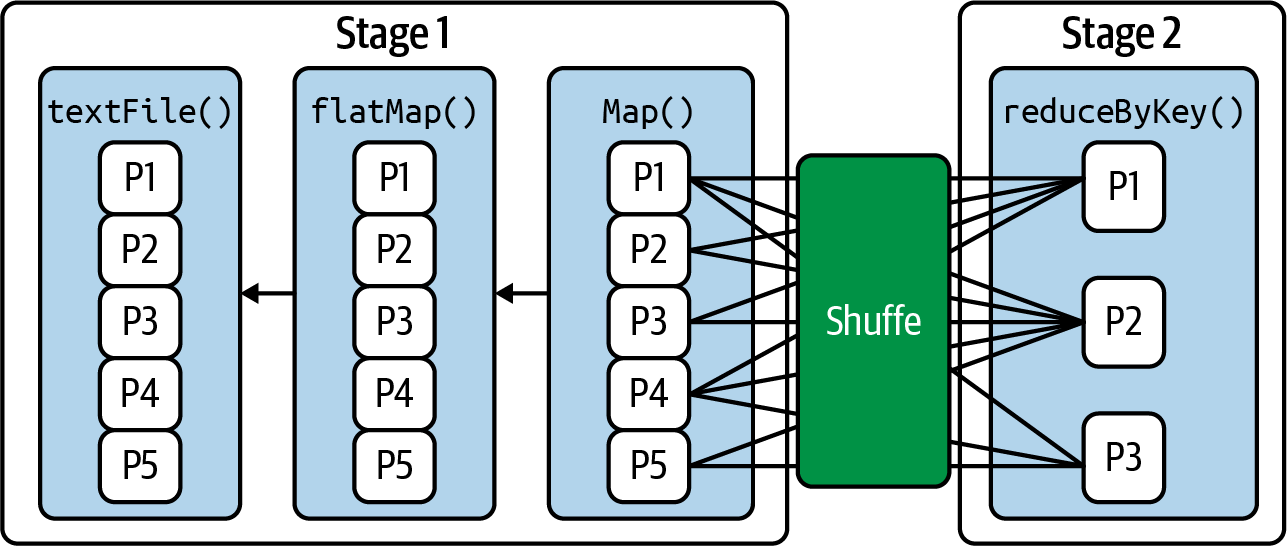
Figure 4-7. Spark’s shuffle concept
Since
shuffling involves copying data across
executors and servers, this
is a complex and costly operation. Let’s take a closer look at how it works for two Spark reduction transformations, groupByKey() and reduceByKey(). This will help illustrate the importance of choosing the appropriate reduction.
Shuffle Step for groupByKey()
The groupByKey() shuffle step is
pretty straightforward. It does not
merge the values for each key; instead, the shuffle happens directly. This means a large volume of data gets sent
to each partition, because there’s no reduction in the initial data values. The
merging of values for each key
happens after the shuffle step. With
groupByKey(), a lot of data needs
to be stored on final worker nodes (reducers), which means you may run into OOM errors if there’s lots of data per key.
Figure 4-8 illustrates the process. Note that after groupByKey(),
you need to call mapValues()
to generate your final desired output.
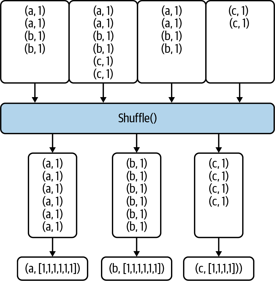
Figure 4-8. Shuffle step for groupByKey()
Because groupByKey() does not merge or combine values, it’s an expensive operation that requires moving large amounts of data over the network.
Shuffle Step for reduceByKey()
With reduceByKey(), the data in each partition is combined so
that there is at most
one value for each key in each partition. Then the shuffle happens, and this data is sent over the network
to the reducers, as illustrated in Figure 4-9. Note that with
reduceByKey(), you do not need need to
call mapValues() to generate your
final desired output. In general, it’s equivalent to using groupByKey() and mapValues(), but because of the reduction in the amount of data sent over the network it is a much more efficient and performant solution.
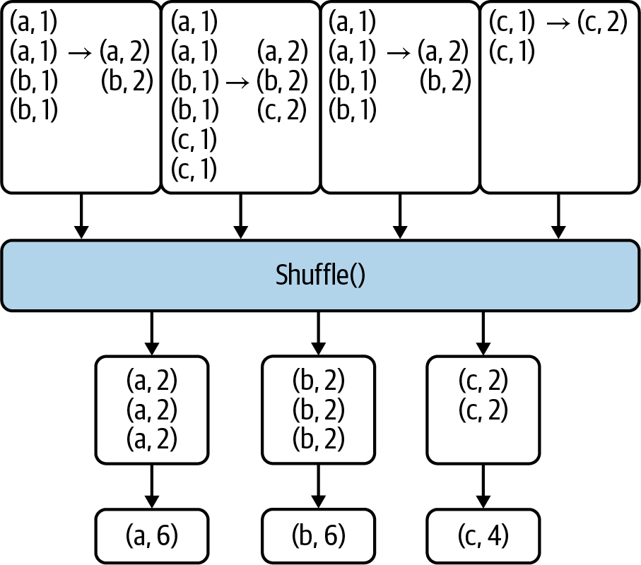
Figure 4-9. Shuffle step for reduceByKey()
Summary
This chapter introduced Spark’s reduction transformations and presented multiple solutions to a real-world data problem with the most commonly used of these transformations: reduceByKey(),
aggregateByKey(), combineByKey(),
and groupByKey(). As you’ve seen,
there are many ways to solve the same
data problem, but they do not all have the same performance.
Table 4-2 summarizes the types of transformations performed by these four reduction transformations (note that V
and C can be different data types).
| Reduction | Source RDD | Target RDD |
|---|---|---|
|
|
|
|
|
|
|
|
|
|
|
|
We learned that some of the reduction transformations
(such as reduceByKey() and combineByKey()) are
preferable over groupByKey(), due to the
shuffle step for groupByKey() being more expensive.
When possible, you should reduceByKey() instead of groupByKey(), or use combineByKey() when you are combining elements but your return type differs from your input value type.
Overall, for large volumes of data, reduceByKey() and
combineByKey() will perform and scale out better than groupByKey().
The aggregateByKey()
transformation is more suitable for aggregations by key that involve computations, such as finding the sum, average, variance, etc. The
important consideration here is that the extra
computation spent for map-side combining can
reduce the amount of data sent out to other worker
nodes and the driver.
In the next chapter we’ll move on to cover partitioning data.
1 For further details, see “Monoidify! Monoids as a Design Principle for Efficient MapReduce Algorithms” by Jimmy Lin.
Get Data Algorithms with Spark now with the O’Reilly learning platform.
O’Reilly members experience books, live events, courses curated by job role, and more from O’Reilly and nearly 200 top publishers.

