Chapter 1. Introduction to Spark and PySpark
Spark is a powerful analytics engine for large-scale data processing that aims at speed, ease of use, and extensibility for big data applications. It’s a proven and widely adopted technology used by many companies that handle big data every day. Though Spark’s “native” language is Scala (most of Spark is developed in Scala), it also provides high-level APIs in Java, Python, and R.
In this book we’ll be using Python via PySpark, an API that exposes the Spark programming model to Python. With Python being the most accessible programming language and Spark’s powerful and expressive API, PySpark’s simplicity makes it the best choice for us. PySpark is an interface for Spark in the Python programming language that provides the following two important features:
-
It allows us to write Spark applications using Python APIs.
-
It provides the PySpark shell for interactively analyzing data in a distributed environment.
The purpose of this chapter is to introduce PySpark as the main component of the Spark ecosystem and show you that it can be effectively used for big data tasks such as ETL operations, indexing billions of documents, ingesting millions of genomes, machine learning, graph data analysis, DNA data analysis, and much more. I’ll start by reviewing the Spark and PySpark architectures, and provide examples to show the expressive power of PySpark. I will present an overview of Spark’s core functions (transformations and actions) and concepts so that you are empowered to start using Spark and PySpark right away. Spark’s main data abstractions are resilient distributed datasets (RDDs), DataFrames, and Datasets. As you’ll see, you can represent your data (stored as Hadoop files, Amazon S3 objects, Linux files, collection data structures, relational database tables, and more) in any combinations of RDDs and DataFrames.
Once your data is represented as a Spark data
abstraction, you can apply transformations on it and
create new data abstractions until the data is in the final form that you’re looking for. Spark’s transformations
(such as map() and reduceByKey()) can be used
to convert your data from one form to another until you get your desired result. I will
explain these data abstractions shortly, but first, let’s dig a little deeper into why Spark is the best choice for data analytics.
Why Spark for Data Analytics
Spark is a powerful analytics engine that can be used for large-scale data processing. The most important reasons for using Spark are:
-
Spark is simple, powerful, and fast.
-
Spark is free and open source.
-
Spark runs everywhere (Hadoop, Mesos, Kubernetes, standalone, or in the cloud).
-
Spark can read/write data from/to any data source (Amazon S3, Hadoop HDFS, relational databases, etc.).
-
Spark can be integrated with almost any data application.
-
Spark can read/write data in row-based (such as Avro) and column-based (such as Parquet and ORC) formats.
-
Spark has a rich but simple set of APIs for all kinds of ETL processes.
In the past five years Spark has progressed in such a way that I believe it can be used to solve any big data problem. This is supported by the fact that all big data companies, such as Facebook, Illumina, IBM, and Google, use Spark every day in production systems.
Spark is one of the best choices for large-scale data processing and for solving MapReduce problems and beyond, as it unlocks the power of data by handling big data with powerful APIs and speed. Using MapReduce/Hadoop to solve big data problems is complex, and you have to write a ton of low-level code to solve even primitive problems—this is where the power and simplicity of Spark comes in. Apache Spark is considerably faster than Apache Hadoop because it uses in-memory caching and optimized execution for fast performance, and it supports general batch processing, streaming analytics, machine learning, graph algorithms, and SQL queries.
For PySpark, Spark has two fundamental data abstractions: the RDD and the DataFrame. I will teach you how to read your data and represent it as an RDD (a set of elements of the same type) or a DataFrame (a table of rows with named columns); this allows you to impose a structure onto a distributed collection of data, permitting higher-level abstraction. Once your data is represented as an RDD or a DataFrame, you may apply transformation functions (such as mappers, filters, and reducers) on it to transform your data into the desired form. I’ll present many Spark transformations that you can use for ETL processes, analysis, and data-intensive computations.
Some simple RDD transformations are represented in Figure 1-1.
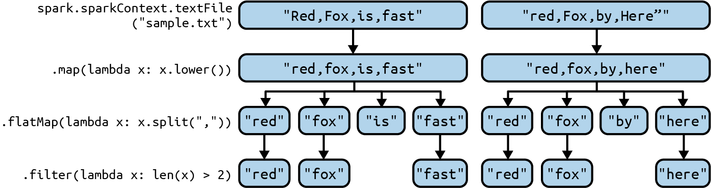
Figure 1-1. Simple RDD transformations
This figure shows the following transformations:
-
First we read our input data (represented as a text file, sample.txt—here, I only show the first two rows/records of input data) with an instance of
SparkSession, which is the entry point to programming Spark. TheSparkSessioninstance is represented as asparkobject. Reading input creates a new RDD as anRDD[String]: each input record is converted to an RDD element of the typeString(if your input path hasNrecords, then the number of RDD elements isN). This is accomplished by the following code:# Create an instance of SparkSessionspark=SparkSession.builder.getOrCreate()# Create an RDD[String], which represents all input# records; each record becomes an RDD elementrecords=spark.sparkContext.textFile("sample.txt") -
Next, we convert all characters to lowercase letters. This is accomplished by the
map()transformation, which is a 1-to-1 transformation:# Convert each element of the RDD to lowercase# x denotes a single element of the RDD# records: source RDD[String]# records_lowercase: target RDD[String]records_lowercase=records.map(lambdax:x.lower()) -
Then, we use a
flatMap()transformation, which is a 1-to-many transformation, to convert each element (representing a single record) into a sequence of target elements (each representing a word). TheflatMap()transformation returns a new RDD by first applying a function (here,split(",")) to all elements of the source RDD and then flattening the results:# Split each record into a list of words# records_lowercase: source RDD[String]# words: target RDD[String]words=records_lowercase.flatMap(lambdax:x.split(",")) -
Finally, we drop word elements with a length less than or equal to 2. The following
filter()transformation drops unwanted words, keeping only those with a length greater than 2:# Keep words with a length greater than 2# x denotes a word# words: source RDD[String]# filtered: target RDD[String]filtered=words.filter(lambdax:len(x)>2)
As you can observe, Spark transformations are high-level, powerful, and simple. Spark is by nature distributed and parallel: your input data is partitioned and can be processed by transformations (such as mappers, filters, and reducers) in parallel in a cluster environment. In a nutshell, to solve a data analytics problem in PySpark, you read data and represent it as an RDD or DataFrame (depending on the nature of the data format), then write a set of transformations to convert your data into the desired output. Spark automatically partitions your DataFrames and RDDs and distributes the partitions across different cluster nodes. Partitions are the basic units of parallelism in Spark. Parallelism is what allows developers to perform tasks on hundreds of computer servers in a cluster in parallel and independently. A partition in Spark is a chunk (a logical division) of data stored on a node in the cluster. DataFrames and RDDs are collections of partitions. Spark has a default data partitioner for RDDs and DataFrames, but you may override that partitioning with your own custom programming.
Next, let’s dive a little deeper into Spark’s ecosystem and architecture.
The Spark Ecosystem
Spark’s ecosystem is presented in Figure 1-2. It has three main components:
- Environments
-
Spark can run anywhere and integrates well with other environments.
- Applications
-
Spark integrates well with a variety of big data platforms and applications.
- Data sources
-
Spark can read and write data from and to many data sources.
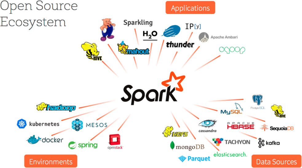
Figure 1-2. The Spark ecosystem (source: Databricks)
Spark’s expansive
ecosystem makes PySpark a
great tool for ETL, data analysis, and many other tasks. With PySpark, you can read data from many different data sources (the Linux
filesystem, Amazon S3, the Hadoop Distributed
File System, relational tables, MongoDB,
Elasticsearch, Parquet files, etc.) and
represent it as a Spark data
abstraction, such as RDDs or DataFrames. Once your data is in that form, you can use
a series of simple and powerful Spark
transformations to transform the data into
the desired shape and format. For example,
you may use the filter() transformation to
drop unwanted records, use groupByKey() to
group your data by your desired key, and
finally use the mapValues() transformation
to perform final aggregation (such as finding
average, median, and standard deviation of
numbers) on the grouped data. All of these
transformations are very possible by using
the simple but powerful PySpark API.
Spark Architecture
When you have small data, it is possible to analyze it with a single computer in a reasonable amount of time. When you have large volumes of data, using a single computer to analyze and process that data (and store it) might be prohibitively slow, or even impossible. This is why we want to use Spark.
Spark has a core library and a set of built-in libraries (SQL, GraphX, Streaming, MLlib), as shown in Figure 1-3. As you can see, through its DataSource API, Spark can interact with many data sources, such as Hadoop, HBase, Amazon S3, Elasticsearch, and MySQL, to mention a few.

Figure 1-3. Spark libraries
This figure shows the real power of Spark: you can use several different languages to write your Spark applications, then use rich libraries to solve assorted big data problems. Meanwhile, you can read/write data from a variety of data sources.
Key Terms
To understand Spark’s architecture, you’ll need to understand a few key terms:
SparkSession-
The
SparkSessionclass, defined in thepyspark.sqlpackage, is the entry point to programming Spark with the Dataset and DataFrame APIs. In order to do anything useful with a Spark cluster, you first need to create an instance of this class, which gives you access to an instance ofSparkContext.Note
PySpark has a comprehensive API (comprised of packages, modules, classes, and methods) to access the Spark API. It is important to note that all Spark APIs, packages, modules, classes, and methods discussed in this book are PySpark-specific. For example, when I refer to the
SparkContextclass I am referring to thepyspark.SparkContextPython class, defined in thepysparkpackage, and when I refer to theSparkSessionclass, I am referring to thepyspark.sql.SparkSessionPython class, defined in thepyspark.sqlmodule. SparkContext-
The
SparkContextclass, defined in thepysparkpackage, is the main entry point for Spark functionality. ASparkContextholds a connection to the Spark cluster manager and can be used to create RDDs and broadcast variables in the cluster. When you create an instance ofSparkSession, theSparkContextbecomes available inside your session as an attribute,SparkSession.sparkContext. - Driver
-
All Spark applications (including the PySpark shell and standalone Python programs) run as independent sets of processes. These processes are coordinated by a
SparkContextin a driver program. To submit a standalone Python program to Spark, you need to write a driver program with the PySpark API (or Java or Scala). This program is in charge of the process of running themain()function of the application and creating theSparkContext. It can also be used to create RDDs and DataFrames. - Worker
-
In a Spark cluster environment, there are two types of nodes: one (or two, for high availability) master and a set of workers. A worker is any node that can run programs in the cluster. If a process is launched for an application, then this application acquires executors at worker nodes, which are responsible for executing Spark tasks.
- Cluster manager
-
The “master” node is known as the cluster manager. The main function of this node is to manage the cluster environment and the servers that Spark will leverage to execute tasks. The cluster manager allocates resources to each application. Spark supports five types of cluster managers, depending on where it’s running:
-
Standalone (Spark’s own built-in clustered environment)
-
Mesos (a distributed systems kernel)
-
Note
While use of master/worker terminology is outmoded and being retired in many software contexts, it is still part of the functionality of Apache Spark, which is why I use this terminology in this book.
Spark architecture in a nutshell
A high-level view of the Spark architecture is presented in Figure 1-4. Informally, a Spark cluster is comprised of a master node (the “cluster manager”), which is responsible for managing Spark applications, and a set of “worker” (executor) nodes, which are responsible for executing tasks submitted by the Spark applications (your applications, which you want to run on the Spark cluster).
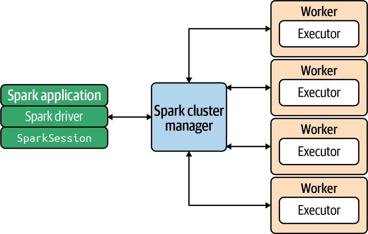
Figure 1-4. Spark architecture
Depending on the environment Spark is running in, the cluster manager managing this cluster of servers will be either Spark’s standalone cluster manager, Kubernetes, Hadoop YARN, or Mesos. When the Spark cluster is running, you can submit Spark applications to the cluster manager, which will grant resources to your application so that you can complete your data analysis.
Your cluster may have one, tens, hundreds, or even thousands of worker nodes, depending on the needs of your business and your project requirements. You can run Spark on a standalone server such as a MacBook, Linux, or Windows PC, but typically for production environments Spark is run on cluster of Linux servers. To run a Spark program, you need to have access to a Spark cluster and have a driver program, which declares the transformations and actions on RDDs of data and submits such requests to the cluster manager. In this book, all driver programs will be in PySpark.
When you start a PySpark shell (by executing
<spark-installed-dir>/bin/pyspark), you
automatically get two variables/objects defined:
spark-
An instance of
SparkSession, which is ideal for creating DataFrames sc-
An instance of
SparkContext, which is ideal for creating RDDs
If you write a self-contained PySpark application
(a Python driver, which uses the PySpark API), then you
have to explicitly create an instance of
SparkSession yourself. A SparkSession
can be used to:
-
Create DataFrames
-
Register DataFrames as tables
-
Execute SQL over tables and cache tables
-
Read/write text, CSV, JSON, Parquet, and other file formats
-
Read/write relational database tables
PySpark defines SparkSession as:
pyspark.sql.SparkSession(Pythonclass,inpyspark.sqlmodule)classpyspark.sql.SparkSession(sparkContext,jsparkSession=None)
SparkSession: the entry point to programming Spark with the RDD
and DataFrame API.
To create a SparkSession in Python, use the
builder pattern shown here:
# import required Spark classfrompyspark.sqlimportSparkSession# create an instance of SparkSession as sparkspark=SparkSession.builder\.master("local")\.appName("my-application-name")\.config("spark.some.config.option","some-value")\.getOrCreate()# to debug the SparkSession(spark.version)# create a reference to SparkContext as sc# SparkContext is used to create new RDDssc=spark.sparkContext# to debug the SparkContext(sc)

Imports the
SparkSessionclass from thepyspark.sqlmodule.
Provides access to the Builder API used to construct
SparkSessioninstances.
Sets a
configoption. Options set using this method are automatically propagated to bothSparkConfand theSparkSession’s own configuration. When creating aSparkSessionobject, you can define any number ofconfig(<key>, <value>)options.
Gets an existing
SparkSessionor, if there isn’t one, creates a new one based on the options set here.
For debugging purposes only.

A
SparkContextcan be referenced from an instance ofSparkSession.
PySpark defines SparkContext as:
classpyspark.SparkContext(master=None,appName=None,...)
SparkContext: the main entry point for Spark functionality.
A SparkContext represents the connection to a Spark cluster,
and can be used to create RDD (the main data abstraction for
Spark) and broadcast variables (such as collections and data
structures) on that cluster.
SparkContext is the main entry point for Spark
functionality. A shell (such as the PySpark shell)
or PySpark driver program cannot create more
than one instance of SparkContext. A SparkContext
represents the connection to a Spark cluster, and
can be used to create new RDDs and broadcast
variables (shared data structures and collections—kind of read-only global variables) on that
cluster. Figure 1-5 shows how a SparkContext can be used to create a new RDD
from an input text file (labeled records_rdd)
and then transform it into another RDD (labeled words_rdd) using
the flatMap() transformation. As you can observe,
RDD.flatMap(f) returns a new RDD by first
applying a function (f) to all elements of
the source RDD, and then flattening the results.
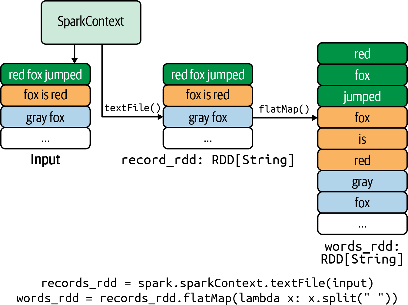
Figure 1-5. Creation of RDDs by SparkContext
To create SparkSession and SparkContext
objects, use the following pattern:
# create an instance of SparkSessionspark_session=SparkSession.builder.getOrCreate()# use the SparkSession to access the SparkContextspark_context=spark_session.sparkContext
If you will be working only with RDDs,
you can create an instance of
SparkContext as follows:
frompysparkimportSparkContextspark_context=SparkContext("local","myapp");
Now that you know the basics of Spark, let’s dive a little deeper into PySpark.
The Power of PySpark
PySpark is a Python API for Apache Spark, designed to support collaboration between Spark and the Python programming language. Most data scientists already know Python, and PySpark makes it easy for them to write short, concise code for distributed computing using Spark. In a nutshell, it’s an all-in-one ecosystem that can handle complex data requirements with its support for RDDs, DataFrames, GraphFrames, MLlib, SQL, and more.
I’ll show you the amazing power of PySpark with a simple example. Suppose we have lots of records containing data on URL visits by users (collected by a search engine from many web servers) in the following format:
<url_address><,><frequency>
Here are a few examples of what these records look like:
http://mapreduce4hackers.com,19779
http://mapreduce4hackers.com,31230
http://mapreduce4hackers.com,15708
...
https://www.illumina.com,87000
https://www.illumina.com,58086
...
Let’s assume we want to find the average,
median, and standard deviation of the
visit numbers per key (i.e., url_address). Another requirement is that we want to drop any records with a length less than 5 (as these may be malformed URLs). It is easy to express an
elegant solution for this in PySpark, as Figure 1-6 illustrates.
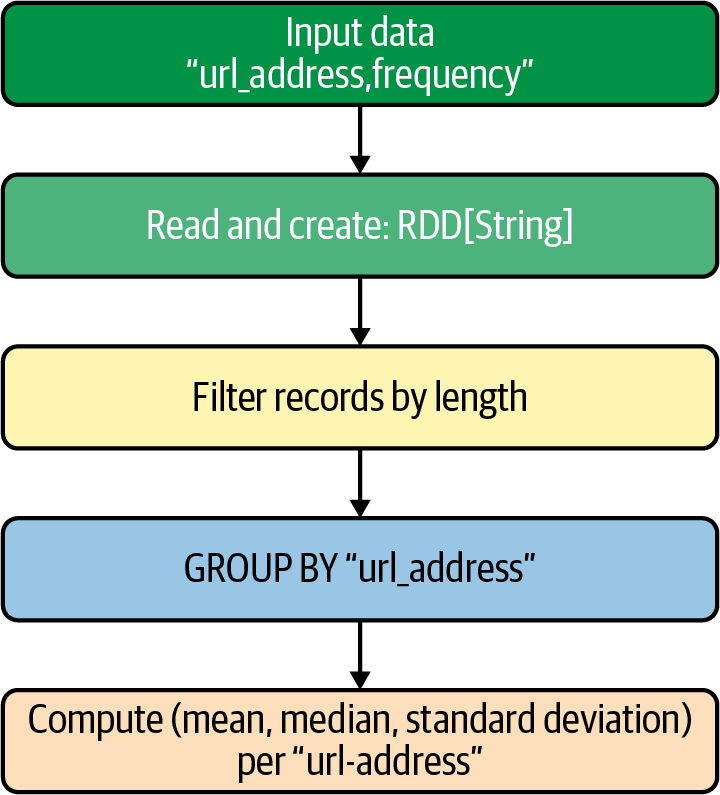
Figure 1-6. Simple workflow to compute mean, median, and standard deviation
First, let’s create some basic Python functions that will help us in solving our simple problem.
The first function, create_pair(), accepts a single
record of the form <url_address><,><frequency> and returns a
(key, value) pair (which will enable us to do a
GROUP BY on the key field later), where the key is
a url_address and the value is the associated frequency:
# Create a pair of (url_address, frequency)# where url_address is a key and frequency is a value# record denotes a single element of RDD[String]# record: <url_address><,><frequency>defcreate_pair(record):tokens=record.split(',')url_address=tokens[0]frequency=tokens[1]return(url_address,frequency)#end-def
Accept a record of the form
<url_address><,><frequency>.Tokenize the input record, using the
url_addressas a key (tokens[0]) and thefrequencyas a value (tokens[1]).Return a pair of
(url_address, frequency).
The next function, compute_stats(), accepts a list of frequencies
(as numbers) and computes three values, the average,
median, and standard deviation:
# Compute average, median, and standard# deviation for a given set of numbersimportstatistics# frequencies = [number1, number2, ...]defcompute_stats(frequencies):average=statistics.mean(frequencies)median=statistics.median(frequencies)standard_deviation=statistics.stdev(frequencies)return(average,median,standard_deviation)#end-def
This module provides functions for calculating mathematical statistics of numeric data.
Accept a list of frequencies.
Compute the average of the frequencies.
Compute the median of the frequencies.
Compute the standard deviation of the frequencies.
Return the result as a triplet.
Next, I’ll show you the amazing power of PySpark in just few lines of code, using Spark transformations and our custom Python functions:
# input_path = "s3://<bucket>/key"input_path="/tmp/myinput.txt"results=spark.sparkContext.textFile(input_path).filter(lambdarecord:len(record)>5).map(create_pair).groupByKey().mapValues(compute_stats)
sparkdenotes an instance ofSparkSession, the entry point to programming Spark.sparkContext(an attribute ofSparkSession) is the main entry point for Spark functionality.Read data as a distributed set of
Stringrecords (creates anRDD[String]).Drop records with a length less than or equal to 5 (keep records with a length greater than 5).
Create
(url_address, frequency)pairs from the input records.Group the data by keys—each key (a
url_address) will be associated with a list of frequencies.
Apply the
compute_stats()function to the list of frequencies.
The result will be a set of (key, value) pairs of the form:
(url_address, (average, median, standard_deviation))
where url-address is a key and
(average, median, standard_deviation)
is a value.
Note
The most important thing about Spark is that it maximizes concurrency of functions and operations by means of partitioning data. Consider an example:
If your input data has 600 billion
rows and you are using a cluster of 10 nodes,
your input data will be partitioned into N
( > 1) chunks, which are processed
independently and in parallel. If N=20,000 (the number of chunks or partitions),
then each chunk will have about 30 million
records/elements (600,000,000,000 / 20,000 = 30,000,000). If you have a big cluster, then
all 20,000 chunks might be processed in one shot. If you
have a smaller cluster, it may be that only every 100
chunks can be processed independently and in
parallel. This process will continue until
all 20,000 chunks are processed.
PySpark Architecture
PySpark is built on top of Spark’s Java API. Data is processed in Python and cached/shuffled in the Java Virtual Machine, or JVM (I will cover the concept of shuffling in Chapter 2). A high-level view of PySpark’s architecture is presented in Figure 1-7.

Figure 1-7. PySpark architecture
And PySpark’s data flow is illustrated in Figure 1-8.
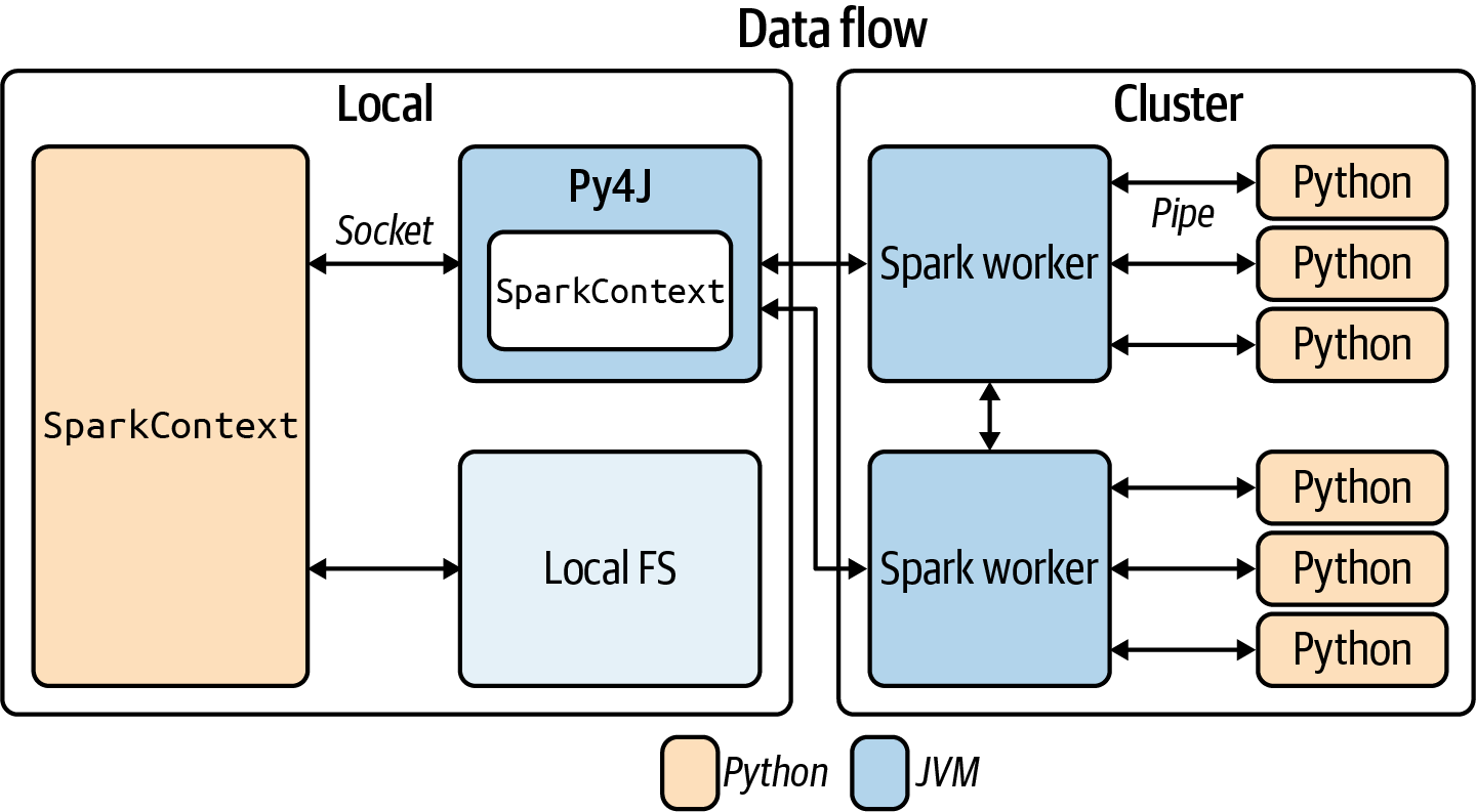
Figure 1-8. PySpark data flow
In the Python driver program (your
Spark application in Python), the SparkContext
uses Py4J
to launch a JVM, creating a
JavaSparkContext. Py4J is only used in
the driver for local communication between
the Python and Java SparkContext objects;
large data transfers are performed through
a different mechanism. RDD transformations
in Python are mapped to transformations on
PythonRDD objects in Java. On remote worker
machines, PythonRDD objects launch Python
subprocesses and communicate with them using
pipes, sending the user’s code and the data
to be processed.
Note
Py4J enables Python programs running in a Python interpreter to dynamically access Java objects in a JVM. Methods are called as if the Java objects resided in the Python interpreter, and Java collections can be accessed through standard Python collection methods. Py4J also enables Java programs to call back Python objects.
Spark Data Abstractions
To manipulate data in the Python programming language, you use integers, strings, lists, and dictionaries. To manipulate and analyze data in Spark, you have to represent it as a Spark dataset. Spark supports three types of dataset abstractions:
-
RDD (resilient distributed dataset):
-
Low-level API
-
Denoted by
RDD[T](each element has typeT)
-
-
DataFrame (similar to relational tables):
-
High-level API
-
Denoted by
Table(column_name_1, column_name_2, ...)
-
-
Dataset (similar to relational tables):
-
High-level API (not available in PySpark)
-
The Dataset data abstraction is used in strongly typed languages such as Java and is not supported in PySpark. RDDs and DataFrames will be discussed in detail in the following chapters, but I’ll give a brief introduction here.
RDD Examples
Essentially, an RDD represents your data as
a collection of elements.
It’s an immutable set of distributed
elements of type T, denoted as RDD[T].
Table 1-1 shows examples of three simple types of RDDs:
RDD[Integer]-
Each element is an
Integer. RDD[String]-
Each element is a
String. RDD[(String, Integer)]-
Each element is a pair of
(String, Integer).
| RDD[Integer] | RDD[String] | RDD[(String, Integer)] |
|---|---|---|
|
|
|
|
|
|
|
|
|
… |
… |
… |
Table 1-2 is an example of a complex RDD. Each element is a (key, value) pair, where the key is a String and the value is a triplet
of (Integer, Integer, Double).
RDD[(String, (Integer, Integer, Double))] |
|---|
|
|
|
|
… |
Spark RDD Operations
Spark RDDs are read-only, immutable, and distributed. Once created, they cannot be altered: you cannot add records, delete records, or update records in an RDD. However, they can be transformed. RDDs support two types of operations: transformations, which transform the source RDD(s) into one or more new RDDs, and actions, which transform the source RDD(s) into a non-RDD object such as a dictionary or array. The relationship between RDDs, transformations, and actions is illustrated in Figure 1-9.
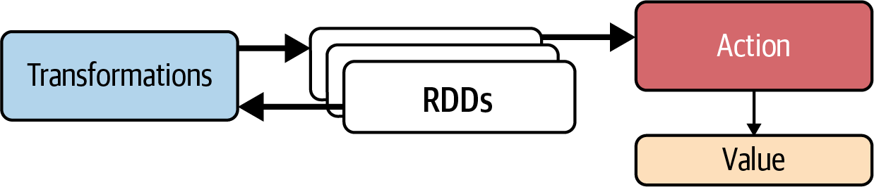
Figure 1-9. RDDs, transformations, and actions
We’ll go into much more detail on Spark’s transformations in the following chapters, with working examples to help you understand them, but I’ll provide a brief introduction here.
Transformations
A transformation in Spark is a function that takes
an existing RDD (the source RDD), applies a
transformation to it, and creates a new RDD (the target
RDD). Examples include: map(),
flatMap(), groupByKey(), reduceByKey(), and
filter().
Informally, we can express a transformation as:
transformation: source_RDD[V] --> target_RDD[T]
Transform
source_RDDof typeVintotarget_RDDof typeT.
RDDs are not evaluated until an action is performed on them: this means that transformations are lazily evaluated. If an RDD fails during a transformation, the data lineage of transformations rebuilds the RDD.
Most Spark transformations create a single RDD, but it is also possible for them to create multiple target RDDs. The target RDD(s) can be smaller, larger, or the same size as the source RDD.
The following example presents a sequence of transformations:
tuples=[('A',7),('A',8),('A',-4),('B',3),('B',9),('B',-1),('C',1),('C',5)]rdd=spark.sparkContext.parallelize(tuples)# drop negative valuespositives=rdd.filter(lambdax:x[1]>0)positives.collect()[('A',7),('A',8),('B',3),('B',9),('C',1),('C',5)]# find sum and average per key using groupByKey()sum_and_avg=positives.groupByKey().mapValues(lambdav:(sum(v),float(sum(v))/len(v)))# find sum and average per key using reduceByKey()# 1. create (sum, count) per keysum_count=positives.mapValues(lambdav:(v,1))# 2. aggregate (sum, count) per keysum_count_agg=sum_count.reduceByKey(lambdax,y:(x[0]+y[0],x[1]+y[1]))# 3. finalize sum and average per keysum_and_avg=sum_count_agg.mapValues(lambdav:(v[0],float(v[0])/v[1]))
Tip
The groupByKey() transformation groups the values for
each key in the RDD into a single sequence, similar to a SQL GROUP BY statement.
This transformation can cause
out of memory (OOM) errors as data is sent over
the network of Spark servers and collected
on the reducer/workers when the number of values
per key is in the thousands or millions.
With the reduceByKey()
transformation, however, data is combined in each
partition, so there is only one output for each key in
each partition to send over the network of
Spark servers. This makes it more scalable than groupByKey(). reduceByKey() merges
the values for each key using an associative
and commutative reduce function. It combines all the values (per key) into another
value with the exact same data type (this is a
limitation, which can be overcome by using the
combineByKey() transformation). Overall,
the reduceByKey() is more scaleable than
the groupByKey(). We’ll talk more about these issues in Chapter 4.
Actions
Spark actions are RDD operations or functions that produce non-RDD values. Informally, we can express an action as:
action: RDD => non-RDD value
Actions may trigger the evaluation of RDDs (which, you’ll recall, are evaluated lazily). However, the output of an action is a tangible value: a saved file, a value such as an integer, a count of elements, a list of values, a dictionary, and so on.
The following are examples of actions:
reduce()-
Applies a function to deliver a single value, such as adding values for a given
RDD[Integer] collect()-
Converts an
RDD[T]into a list of typeT count()-
Finds the number of elements in a given RDD
saveAsTextFile()-
Saves RDD elements to a disk
saveAsMap()-
Saves
RDD[(K, V)]elements to a disk as adict[K, V]
DataFrame Examples
Similar to an RDD, a DataFrame in Spark is an immutable distributed collection of data. But unlike in an RDD, the data is organized into named columns, like a table in a relational database. This is meant to make processing of large datasets easier. DataFrames allow programmers to impose a structure onto a distributed collection of data, allowing higher-level abstraction. They also make the processing of CSV and JSON files much easier than with RDDs.
The following DataFrame example has three columns:
DataFrame[name, age, salary]
name: String, age: Integer, salary: Integer

+-----+----+---------+
| name| age|   salary|
+-----+----+---------+
|  bob|  33|    45000|
| jeff|  44|    78000|
| mary|  40|    67000|
|  ...| ...|      ...|
+-----+----+---------+
A DataFrame can be created from many different sources, such as Hive tables, Structured Data Files (SDF), external databases, or existing RDDs. The DataFrames API was designed for modern big data and data science applications, taking inspiration from DataFrames in R and pandas in Python. As we will see in later chapters, we can execute SQL queries against DataFrames.
Spark SQL comes with an extensive set of powerful DataFrame operations that includes:
-
Aggregate functions (min, max, sum, average, etc.)
-
Collection functions
-
Math functions
-
Sorting functions
-
String functions
-
User-defined functions (UDFs)
For example, you can easily read a CSV file and create a DataFrame from it:
# define input pathvirus_input_path="s3://mybucket/projects/cases/case.csv"# read CSV file and create a DataFramecases_dataframe=spark.read.load(virus_input_path,format="csv",sep=",",inferSchema="true",header="true")# show the first 3 rows of created DataFramecases_dataframe.show(3)+-------+-------+-----------+--------------+---------+|case_id|country|city|infection_case|confirmed|+-------+-------+-----------+--------------+---------+|C0001|USA|NewYork|contact|175|+-------+-------+-----------+--------------+---------+|C0008|USA|NewJersey|unknown|25|+-------+-------+-----------+--------------+---------+|C0009|USA|Cupertino|contact|100|+-------+-------+-----------+--------------+---------+
To sort the results by number of cases in descending order, we can use the sort() function:
# We can do this using the F.desc function:frompyspark.sqlimportfunctionsasFcases_dataframe.sort(F.desc("confirmed")).show()+-------+-------+-----------+--------------+---------+|case_id|country|city|infection_case|confirmed|+-------+-------+-----------+--------------+---------+|C0001|USA|NewYork|contact|175|+-------+-------+-----------+--------------+---------+|C0009|USA|Cupertino|contact|100|+-------+-------+-----------+--------------+---------+|C0008|USA|NewJersey|unknown|25|+-------+-------+-----------+--------------+---------+
We can also easily filter rows:
cases_dataframe.filter((cases_dataframe.confirmed>100)&(cases_dataframe.country=='USA')).show()+-------+-------+-----------+--------------+---------+|case_id|country|city|infection_case|confirmed|+-------+-------+-----------+--------------+---------+|C0001|USA|NewYork|contact|175|+-------+-------+-----------+--------------+---------+...
To give you a better idea of the power of Spark’s DataFrames, let’s walk through an example. We will create a DataFrame and find the average and sum of hours worked by employees per department:
# Import required librariesfrompyspark.sqlimportSparkSessionfrompyspark.sql.functionsimportavg,sum# Create a DataFrame using SparkSessionspark=SparkSession.builder.appName("demo").getOrCreate()dept_emps=[("Sales","Barb",40),("Sales","Dan",20),("IT","Alex",22),("IT","Jane",24),("HR","Alex",20),("HR","Mary",30)]df=spark.createDataFrame(dept_emps,["dept","name","hours"])# Group the same depts together, aggregate their hours, and compute an averageaverages=df.groupBy("dept").agg(avg("hours").alias('average'),sum("hours").alias('total'))# Show the results of the final executionaverages.show()+-----+--------+------+|dept|average|total|+-----+--------+------+|Sales|30.0|60.0||IT|23.0|46.0||HR|25.0|50.0|+-----+--------+------+
As you can see, Spark’s DataFrames are powerful enough to manipulate billions of rows with simple but powerful functions.
Using the PySpark Shell
There are two main ways you can use PySpark:
-
Use the PySpark shell (for testing and interactive programming).
-
Use PySpark in a self-contained application. In this case, you write a Python driver program (say, my_pyspark_program.py) using the PySpark API and then run it with the
spark-submitcommand:export SUBMIT=$SPARK_HOME/bin/spark-submit $SUBMIT [options] my_pyspark_program.py <parameters>
where
<parameters>is a list of parameters consumed by your PySpark (my_pyspark_program.py) program.
Note
For details on using the spark-submit
command, refer to
“Submitting Applications” in the Spark documentation.
In this section we’ll focus on Spark’s interactive shell for Python
users, a powerful tool that you can use to analyze data interactively
and see the results immediately (Spark also provides a Scala shell). The PySpark shell can work on both single-machine installations and cluster installations of Spark. You use the following command to start the shell, where SPARK_HOME denotes the installation directory for Spark on your system:
export SPARK_HOME=<spark-installation-directory>
$SPARK_HOME/bin/pyspark
For example:
export SPARK_HOME="/home/spark"
Define the Spark installation directory.
Invoke the PySpark shell.
When you start the shell,
PySpark displays some useful information including details on the Python and Spark versions it is using (note that the output here has been shortened).
The >>> symbol is used as the PySpark shell prompt.
This prompt indicates that you can now
write Python or PySpark commands and view
the results.
To get you comfortable with the PySpark shell, the following sections will walk you through some basic usage examples.
Launching the PySpark Shell
To enter into a PySpark shell, we execute pyspark as follows:
$SPARK_HOME/bin/pyspark
Welcome to
      ____              __
     / __/__  ___ _____/ /__
    _\ \/ _ \/ _ `/ __/  '_/
   /__ / .__/\_,_/_/ /_/\_\   version 3.1.2
      /_/

SparkSession available as 'spark'.
SparkContext available as 'sc'.
>>>sc.version'3.1.2'>>>spark.version'3.1.2'
Executing
pysparkwill create a new shell. The output here has been shortened.Verify that
SparkContextis created assc.Verify that
SparkSessionis created asspark.
Once you enter into the PySpark shell, an instance
of SparkSession is created as the spark variable
and an instance of SparkContext is created as the sc variable. As you learned earlier in this chapter, the SparkSession is the entry
point to programming Spark with the Dataset and
DataFrame APIs; a SparkSession can be used to
create DataFrames, register DataFrames as tables,
execute SQL over tables, cache tables, and
read CSV, JSON, and Parquet files.
If you want to use PySpark in a self-contained
application, then you have to explicitly create
a SparkSession using the builder pattern shown in “Spark architecture in a nutshell”.
A SparkContext is the main entry point for Spark functionality; it can be used to
create RDDs from text files and Python
collections. We’ll look at that next.
Creating an RDD from a Collection
Spark enables us to create new RDDs from files
and collections (data structures such as arrays and lists).
Here, we use SparkContext.parallelize() to
create a new RDD from a collection (represented
as data):
>>>data=[("fox",6),("dog",5),("fox",3),("dog",8),("cat",1),("cat",2),("cat",3),("cat",4)]>>># use SparkContext (sc) as given by the PySpark shell>>># create an RDD as rdd>>>rdd=sc.parallelize(data)>>>rdd.collect()[('fox',6),('dog',5),('fox',3),('dog',8),('cat',1),('cat',2),('cat',3),('cat',4)]>>>rdd.count()8
Define your Python collection.
Create a new RDD from a Python collection.
Display the contents of the new RDD.
Count the number of elements in the RDD.
Aggregating and Merging Values of Keys
The reduceByKey() transformation is
used to merge and aggregate values.
In this example, x and y
refer to the values of the same key:
>>>sum_per_key=rdd.reduceByKey(lambdax,y:x+y)>>>sum_per_key.collect()[('fox',9),('dog',13),('cat',10)]
Merge and aggregate values of the same key.
Collect the elements of the RDD.
The source RDD for this transformation must consist of (key, value) pairs. reduceByKey()
merges the values for each key using an
associative and commutative reduce function.
This will also perform the merging locally
on each mapper before sending the results to a
reducer, similarly to a “combiner” in MapReduce.
The output will
be partitioned with numPartitions
partitions, or the default parallelism level
if numPartitions is not specified. The default
partitioner is HashPartitioner.
If T is the type of the value for (key, value) pairs,
then reduceByKey()’s func() can be defined as:
# source_rdd : RDD[(K, T)]# target_rdd : RDD[(K, T)]target_rdd=source_rdd.reduceByKey(lambdax,y:func(x,y))# OR you may write it by passing the function name# target_rdd = source_rdd.reduceByKey(func)# where# func(T, T) -> T# Then you may define `func()` in Python as:# x: type of T# y: type of Tdeffunc(x,y):result=<aggregationofxandy:returnaresultoftypeT>returnresult#end-def
This means that:
-
There are two input arguments (of the same type,
T) for the reducerfunc(). -
The return type of
func()must be the same as the input typeT(this limitation can be avoided if you use thecombineByKey()transformation). -
The reducer
func()has to be associative. Informally, a binary operationf()on a setTis called associative if it satisfies the associative law, which states that the order in which numbers are grouped does not change the result of the operation. -
The reducer
func()has to be commutative: informally, a functionf()for whichf(x, y) = f(y, x)for all values ofxandy. That is, a change in the order of the numbers should not affect the result of the operation.Commutative Law
f(x, y) = f(y, x)
The commutative law also holds for addition and multiplication, but not for subtraction or division. For example:
5 + 3 = 3 + 5 but 5 – 3 ≠ 3 – 5
Therefore, you may not use subtraction or division
operations in a reduceByKey() transformation.
Filtering an RDD’s Elements
Next, we’ll use the filter() transformation to
return a new RDD containing only the elements
that satisfy a predicate:
>>>sum_filtered=sum_per_key.filter(lambdax:x[1]>9)>>>sum_filtered.collect()[('cat',10),('dog',13)]
Keep the (key, value) pairs if the value is greater than 9.
Collect the elements of the RDD.
Grouping Similar Keys
We can use the groupByKey() transformation to group the values for each key in the RDD
into a single sequence:
>>>grouped=rdd.groupByKey()>>>grouped.collect()[('fox',<ResultIterableobjectat0x10f45c790>),('dog',<ResultIterableobjectat0x10f45c810>),('cat',<ResultIterableobjectat0x10f45cd90>)]>>>>>># list(v) converts v as a ResultIterable into a list>>>grouped.map(lambda(k,v):(k,list(v))).collect()[('fox',[6,3]),('dog',[5,8]),('cat',[1,2,3,4])]
Group elements of the same key into a sequence of elements.
View the result.
The full name of
ResultIterableispyspark.resultiterable.ResultIterable.First apply
map()and thencollect(), which returns a list that contains all of the elements in the resulting RDD. Thelist()function convertsResultIterableinto a list of objects.
The source RDD for this transformation must be composed of (key, value) pairs. groupByKey()
groups the values for each key in the RDD
into a single sequence, and hash-partitions the
resulting RDD with numPartitions partitions, or with the default level of parallelism if numPartitions is not specified.
Note that if you are grouping (using the
groupByKey() transformation) in order to
perform an aggregation, such as a sum or
average, over each key, using reduceByKey()
or aggregateByKey() will provide much better
performance.
Aggregating Values for Similar Keys
To aggregate and sum up the values for each
key, we can use the mapValues() transformation
and the sum() function:
>>>aggregated=grouped.mapValues(lambdavalues:sum(values))>>>aggregated.collect()[('fox',9),('dog',13),('cat',10)]
valuesis a sequence of values per key. We pass each value in the (key, value) pair RDD through a mapper function (adding allvalueswithsum(values)) without changing the keys.For debugging, we return a list that contains all of the elements in this RDD.
We have several choices for aggregating and summing
up values: reduceByKey()
and groupByKey(), to mention a few. In general, the
reduceByKey() transformation is more efficient than
the groupByKey() transformation. More details on this are provided in Chapter 4.
As you’ll see in the following chapters, Spark has many other powerful transformations that can convert an RDD into a new RDD. As mentioned earlier, RDDs are read-only, immutable, and distributed. RDD transformations return a pointer to a new RDD and allow you to create dependencies between RDDs. Each RDD in the dependency chain (or string of dependencies) has a function for calculating its data and a pointer (dependency) to its parent RDD.
Data Analysis Tools for PySpark
- Jupyter
-
Jupyter is a great tool to test and prototype programs. PySpark can also be used from Jupyter notebooks; it’s very practical for explorative data analysis.
- Apache Zeppelin
-
Zeppelin is a web-based notebook that enables data-driven, interactive data analytics and collaborative documents with SQL, Python, Scala, and more.
ETL Example with DataFrames
In data analysis and computing, ETL is the general procedure of copying data from one or more sources into a destination system that represents the data differently from the source(s) or in a different context than the source(s). Here I will show how Spark makes ETL possible and easy.
For this ETL example, I’ll use 2010 census data in JSON format (census_2010.json):
$ wc -l census_2010.json
101 census_2010.json

$ head -5 census_2010.json
{"females": 1994141, "males": 2085528, "age": 0, "year": 2010}
{"females": 1997991, "males": 2087350, "age": 1, "year": 2010}
{"females": 2000746, "males": 2088549, "age": 2, "year": 2010}
{"females": 2002756, "males": 2089465, "age": 3, "year": 2010}
{"females": 2004366, "males": 2090436, "age": 4, "year": 2010}
Note
This data was pulled from U.S. Census Bureau data, which at the time of writing this book only provides the binary options of male and female. We strive to be as inclusive as possible, and hope that in the future national data sets such as these will provide more inclusive options.
Let’s define our ETL process:
- Extraction
-
First, we create a DataFrame from a given JSON document.
- Transformation
-
Then we filter the data and keep the records for seniors (
age > 54). Next, we add a new column,total, which is the total of males and females. - Loading
-
Finally, we write the revised DataFrame into a MySQL database and verify the load process.
Let’s dig into this process a little more deeply.
Extraction
To do a proper extraction, we first need to create an
instance of the SparkSession class:
frompyspark.sqlimportSparkSessionspark=SparkSession.builder\.master("local")\.appName("ETL")\.getOrCreate()
Next, we read the JSON and create a DataFrame:
>>>input_path="census_2010.json">>>census_df=spark.read.json(input_path)>>>census_df.count()101>>>census_df.show(200)+---+-------+-------+----+|age|females|males|year|+---+-------+-------+----+|0|1994141|2085528|2010||1|1997991|2087350|2010||2|2000746|2088549|2010|...|54|2221350|2121536|2010||55|2167706|2059204|2010||56|2106460|1989505|2010|...|98|35778|8321|2010||99|25673|4612|2010|+---+-------+-------+----+onlyshowingtop100rows
Transformation
Transformation can involve many processes whose purpose is to clean, format, or perform computations on the data to suit your requirements. For example, you can remove missing or duplicate data, join columns to create new columns, or filter out certain rows or columns. Once we’ve created the DataFrame through the extraction process, we can perform many useful transformations, such as selecting just the seniors:
>>>seniors=census_df[census_df['age']>54]>>>seniors.count()46>>>seniors.show(200)+---+-------+-------+----+|age|females|males|year|+---+-------+-------+----+|55|2167706|2059204|2010||56|2106460|1989505|2010||57|2048896|1924113|2010|...|98|35778|8321|2010||99|25673|4612|2010||100|51007|9506|2010|+---+-------+-------+----+
Next, we create a new aggregated column called total,
which adds up the numbers of males and females:
>>>frompyspark.sql.functionsimportlit>>>seniors_final=seniors.withColumn('total',lit(seniors.males+seniors.females))>>>seniors_final.show(200)+---+-------+-------+----+-------+|age|females|males|year|total|+---+-------+-------+----+-------+|55|2167706|2059204|2010|4226910||56|2106460|1989505|2010|4095965||57|2048896|1924113|2010|3973009|...|98|35778|8321|2010|44099||99|25673|4612|2010|30285||100|51007|9506|2010|60513|+---+-------+-------+----+-------+
Loading
The loading process involves saving or writing the
final output of the transformation step. Here, we
will write the seniors_final DataFrame into
a MySQL table:
seniors_final\.write\.format("jdbc")\.option("driver","com.mysql.jdbc.Driver")\.mode("overwrite")\.option("url","jdbc:mysql://localhost/testdb")\.option("dbtable","seniors")\.option("user","root")\.option("password","root_password")\.save()
The final step of loading is to verify the load process:
$mysql-uroot-pEnterpassword:<password>YourMySQLconnectionidis9Serverversion:5.7.30MySQLCommunityServer(GPL)mysql>usetestdb;Databasechangedmysql>select*fromseniors;+------+---------+---------+------+---------+|age|females|males|year|total|+------+---------+---------+------+---------+|55|2167706|2059204|2010|4226910||56|2106460|1989505|2010|4095965||57|2048896|1924113|2010|3973009|...|98|35778|8321|2010|44099||99|25673|4612|2010|30285||100|51007|9506|2010|60513|+------+---------+---------+------+---------+46rowsinset(0.00sec)
Summary
Let’s recap some key points from the chapter:
-
Spark is a fast and powerful unified analytics engine (up to one hundred times faster than traditional Hadoop MapReduce) due to its in-memory operation, and it offers robust, distributed, fault-tolerant data abstractions (called RDDs and DataFrames). Spark integrates with the world of machine learning and graph analytics through the MLlib (machine learning library) and GraphX (graph library) packages.
-
You can use Spark’s transformations and actions in four programming languages: Java, Scala, R, and Python. PySpark (the Python API for Spark) can be used for solving big data problems, efficiently transforming your data into the desired result and format.
-
Big data can be represented using Spark’s data abstractions (RDDs, DataFrames, and Datasets—all of these are distributed datasets).
-
You can run PySpark from the PySpark shell (using the
pysparkcommand from a command line) for interactive Spark programming. Using the PySpark shell, you can create and manipulate RDDs and DataFrames. -
You can submit a standalone PySpark application to a Spark cluster by using the
spark-submitcommand; self-contained applications using PySpark are deployed to production environments. -
Spark offers many transformations and actions for solving big data problems, and their performance differs (for example,
reduceByKey()versusgroupByKey()andcombineByKey()versusgroupByKey()).
The next chapter dives into some important Spark transformations.
Get Data Algorithms with Spark now with the O’Reilly learning platform.
O’Reilly members experience books, live events, courses curated by job role, and more from O’Reilly and nearly 200 top publishers.

