Chapter 4. DNN Processing for Image, Audio, and Video
In Chapter 3, we created a neural network able to classify simple images of items of clothing to illustrate the principles of neural network technology. However, the simplicity of the Fashion-MNIST data meant that it was not a scenario with much realism. DNNs are able to solve far more complex problems through a wide range of architectures other than simple feed-forward, fully connected networks.
There are many different ways of designing a DNN, using different layering structures, different types of layers, and different ways of connecting the nodes. The network will depend upon the task, and these different flavors of DNN may also be combined with each other or other algorithms, enabling them to perform even more complex tasks.
This chapter, therefore, considers how DNN technology can be applied to more realistic image, audio, and video processing. We’ll build on the basics from Chapter 3 to understand the concepts behind the neural networks commonly used in these fields and how these technologies are combined with more traditional processing to get the best results.
This discussion will focus on two key network types: convolutional neural networks (CNNs) and recurrent neural networks (RNNs). These demonstrate common patterns in the context of image and audio processing and also are referenced in discussions later in the book. CNNs and RNNs are not the only DNNs relevant to image, audio, and video processing, but they are the networks in most common use. The descriptions given here are introductory only. If you are interested in learning more about a particular network type, consult the resources available in this book’s GitHub repository.
To understand how DNNs can be used to process image and audio, and to appreciate how the data may be manipulated to create adversarial examples, we must begin with the computational representation of the data. Each section in this chapter, therefore, begins by considering the digital encoding of the data for the particular data type (image, audio, and video). In later chapters, it will become clear how the digital encoding of the data and specifically the precision of that encoding will directly affect the ability to create adversarial input. Alterations to the data precision during data compression or transformation steps might (inadvertently or deliberately) remove adversarial content.
By the time you reach the end of the chapter you’ll have acquired sufficient knowledge of how image, audio, and video are digitally represented, as well as familiarity with common neural network design patterns, to understand the discussions on adversarial examples in the chapters that follow.
Image
At the most basic level, human visual processing enables us to perceive light, a portion of the electromagnetic spectrum with wavelengths in the range of 200 to 700 nanometers. Alternatively, light can be described in terms of frequency, where the frequency of the wave is the inverse of the wavelength. Frequency is measured by number of cycles per second in Hertz (Hz), and light has a frequency range of roughly 430 to 750 terahertz (THz). Lower frequencies correspond to infrared electromagnetic radiation, and higher frequencies correspond to ultraviolet.
Three types of color receptors (“cones”) in our eyes are sensitive to different wavelengths of light. One type of cone is sensitive to longer wavelengths within the visible spectrum (red light), the second to the medium wavelengths (green light), and the third to the shorter wavelengths (blue light). These receptors send signals to the brain when light of the appropriate color wavelength reaches them; so, a cone that is sensitive to light from the blue end of the spectrum will send a signal to the brain when blue light enters the eye, with the magnitude of the signal corresponding to the amount of blue light. Our visual cortex then combines these signals to create the actual color that we perceive.
Digital Representation of Images
Digital images are made of pixels, where each pixel is a discrete value representing the analog light waveform at that point. The Fashion-MNIST images are, obviously, a pretty poor representation of real life. For starters, an image in the Fashion-MNIST database is represented by its monochrome pixel intensities, each pixel having a value between 0 and 255. A pixel value of 0 represents black (minimum intensity), and a pixel value of 255 represents white (maximum intensity). Each value takes exactly 1 byte of storage (because 8 bits can represent 256 possible values).
One approach in showing color images is to represent 256 colors using the same amount of storage. This requires a “color palette”—essentially a mapping to assign each of the 256 values to its allocated color. While this is quite expressive, it still doesn’t provide sufficient variety and range of colors to adequately capture realistic images. Therefore, for photographs, each pixel is typically represented by three values—one for red, one for green, and one for blue. These red-green-blue or RGB values typically are allowed 1 byte of storage each, so each has a value between 0 and 255. To calculate the color of an individual pixel, the RGB values for that pixel are combined. This representation is very flexible; RGB values between 0 and 255 allow a palette of 16,777,216 possible colors. Yes, you guessed it, this notion of creating colors from three separate red, green, and blue inputs was inspired by the cones color receptors in the human eye.
The Fashion-MNIST images are not only monochrome but also extremely low resolution—28 x 28 pixels, a mere 784 pixels per image. Even a relatively low-resolution 0.3 megapixel photograph has approximately 640 x 480 pixels. Cameras nowadays take photographs with far greater pixel accuracy (2 megapixels and above).
The precision of an image is measured by the depth of its color (the number of bits used to indicate the value of each pixel) and the number of pixels. These two attributes are respectively referred to as the color resolution and spatial resolution, as shown in Figure 4-1. Reducing spatial resolution results in less smooth lines. Reducing color resolution results in more blocky textures.
The overall image precision selected will depend upon how it was captured (the camera’s settings), its usage (for example, size of print required), and storage constraints. There are several common image formats used for image processing, but JPEGs (standardized by the Joint Photographic Experts Group) are good for both capturing realism in photos requiring color depth (using RGB blending) and for high pixel resolution.
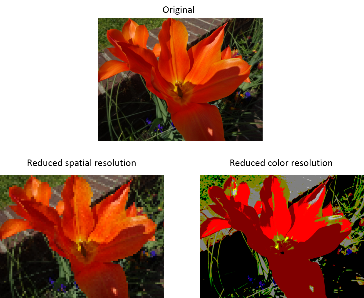
Figure 4-1. The effect of reduced spatial and color resolution on an image
DNNs for Image Processing
The most basic task of image processing is to classify an image based on its primary content, as we did in Chapter 3 for the Fashion-MNIST dataset. Most image processing will be more complex than this, however. For example:
- Scene classification
-
Classification of a scene (such as “beach scene” or “street scene”), rather than classification based on the most prevalent object.
- Object detection and localization
-
Such as detection of faces within an image and establishing where they are in the image.
- Semantic segmentation
-
Fine-grained depiction of regions in the image, corresponding to different classifications. An example is illustrated in Figure 4-2.
- Facial recognition
-
DNNs can be used for facial recognition systems. With sufficient training data, the problem of facial recognition can become simply a classification task, where the number of classifications equals the number of individuals in the dataset. A facial recognition system might be combined with a detection algorithm to extract faces from a scene and recognize them.
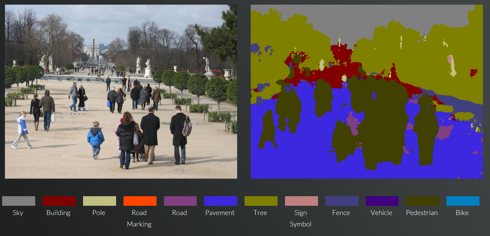
Figure 4-2. An example of image segmentation1
Solutions for some of these tasks using traditional (nonneural network) vision processing techniques have existed for many years. For example, using more traditional image processing techniques, faces can be detected within an image, extracted, and resized, and the data transformed and normalized. Algorithms can then extract the fiducial points of the face—that is, the important values for positioning the face and for facial recognition, such as the corners of the mouth or edges of the eyes. The fiducial measurements can then be exploited to recognize the individual, typically through statistical (including machine learned) approaches. DNNs, however, have enabled a step-change in vision processing capability and accuracy and are replacing, or being used in conjunction with, traditional approaches across image processing.
Introducing CNNs
An underlying challenge with vision processing is understanding the image contents regardless of spatial positioning and size. We avoided this problem in Chapter 3 because each clothing item in the Fashion-MNIST dataset is of roughly the same size, oriented correctly, and placed centrally within the image.
In real life such consistent sizing and positioning within an image is highly unlikely. If a DNN’s predicted probability of a “cat” within an image depends upon the existence of certain “whiskery” aspects of the picture, there is no way of guaranteeing where those whiskery aspects will be located or what size they will be. It will depend upon the size, orientation, and position of the cat. What’s needed is some clever way of extracting patterns from within an image, wherever they are located. When we have extracted patterns, we can use these to perform higher-level image processing.
Extracting spatial patterns within data is exactly what a convolutional neural network is able to do. This means that CNNs are usually the neural networks of choice for image processing tasks.
A CNN is a network that contains one or more convolutional layers—these are layers that use an algorithm to extract features from the image, regardless of their location. A convolutional layer “convolves” one or more filters across every part of the image. In other words, it performs some filtering on a tiny part of the image, then performs the same filtering on an adjacent, overlapping part, and so on until it has covered the complete image. The convolution means moving the filter across the image in small overlapping steps, as shown in Figure 4-3.
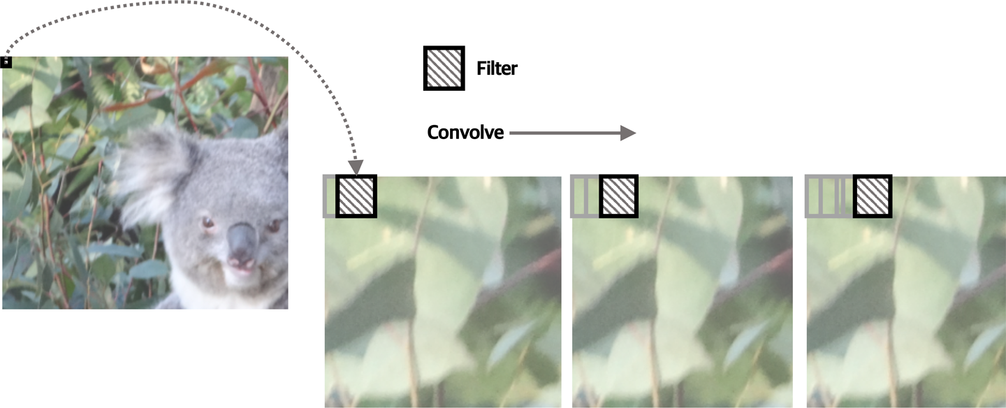
Figure 4-3. A convolutional filter is applied iteratively across an image
As the filter is applied to a small part of the image, it generates a numeric score that indicates how accurately the image part represents the feature filter.
To give you a better idea of how this works, a trivial 3 x 3 filter representing a vertical dark line against a light background is shown in Figure 4-4; it is just a simple matrix of numbers. Examples of its application to two different 3 x 3 pixel segments of a monochrome image are shown. Elementwise multiplication is performed between the feature filter and the image segment (this is simply a case of multiplying the value in each matrix with the corresponding one in the other to create a new matrix). The average (mean) of the values in the resulting matrix is then calculated.
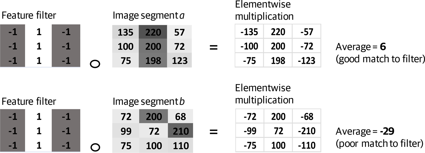
Figure 4-4. Application of a simple 3 x 3 filter to two different image segments
As you can see, the value calculated for image segment a is a relatively high 6, indicating that the image segment represents a little bit of vertical line. The filter output for image segment b is –29, correctly indicating that this part of the image is not representative of a vertical line.
All the values resulting from convolving the filter over the image are placed in an array that will be output from the convolutional layer. This is called a feature map.
In practice, the filters are more complex than those in Figure 4-4, and the values are optimized during training. As with the weights and bias parameters learned in Chapter 3, the filters are typically set randomly and learned. So the convolutional layers learn the important features in the training data, and encapsulate those features within the filter maps.
At this stage, let’s pause and clarify exactly what is passed to, and returned from, a convolutional layer. If the convolutional layer is at the start of the network, it is taking an image as input. For a color image represented by RGB values, this is a 3D array: one dimension for the image’s height, one dimension for its width, and one dimension for each of the red, green, and blue color channels. The 3D “shape” of the data being passed to the neural network for a 224 x 224 pixel image would be:
shape=(224,224,3)
A convolutional layer may apply more than one filter, which means that it will return a stack of feature maps—one for each time a filter is applied across the input. This means that a convolutional layer might generate more data than it consumes! To reduce the dimensionality (and noise) from the output, a convolutional layer is typically followed by a pooling layer. During pooling, small windows of the data are iteratively stepped over (similar to the way the convolution filter “steps” across the image). The data in each window is “pooled” to give a single value. There are several approaches to the pooling step. For example, we might perform pooling by taking the average value of the windowed data, or by taking the maximum value. This latter case of max pooling has the effect of shrinking the data and also relaxing the precision of the filtering if the filter wasn’t a perfect match by discarding lower values.
Typically, the layers in the first part of a CNN alternate in type—convolution, pooling, convolution, pooling, etc. Layers containing simple ReLU functionality might also be incorporated to remove negative values, and these may be logically combined with the convolutional step. Figure 4-5 shows one way that these layers might be organized.
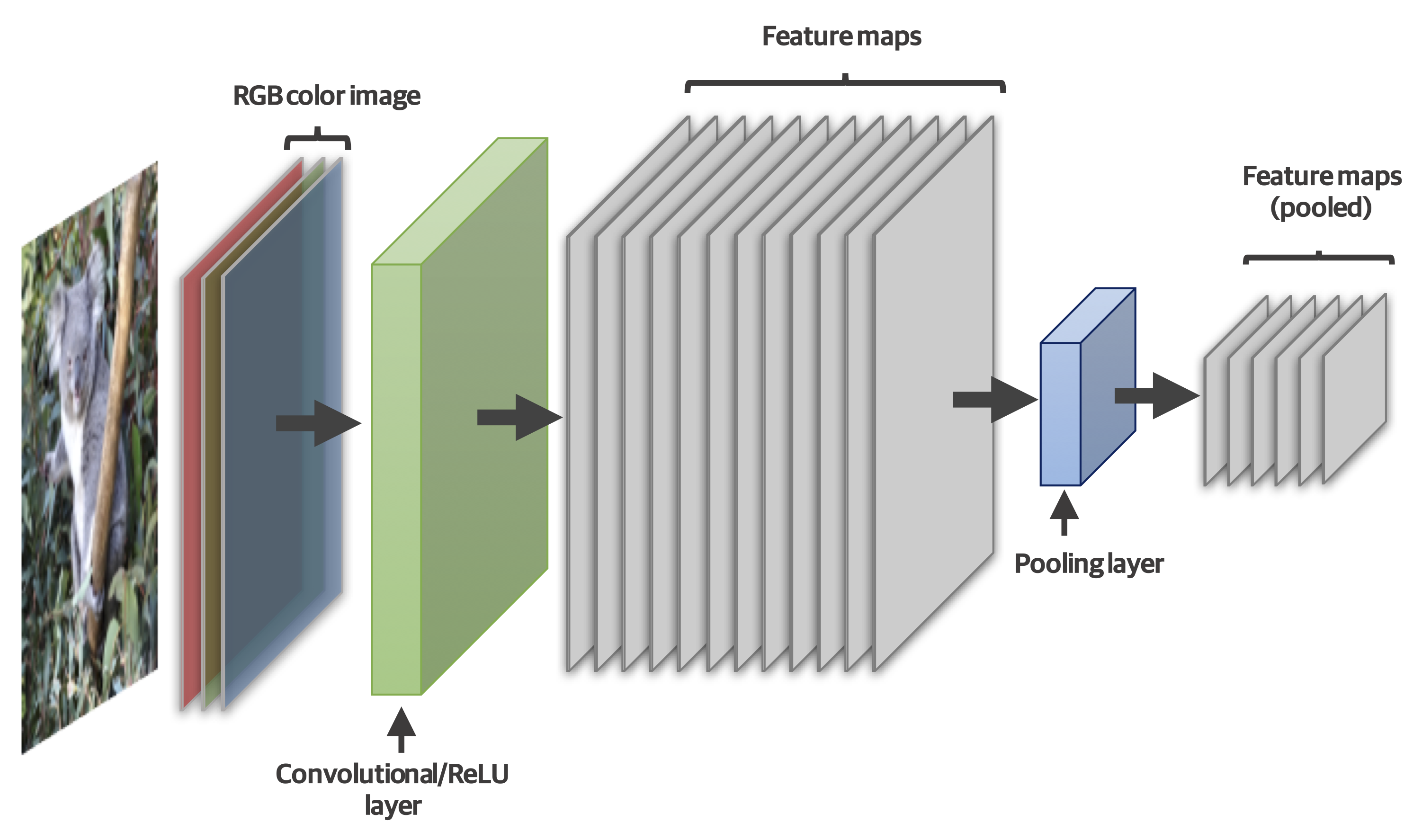
Figure 4-5. Typical layering pattern in a CNN
To see how the convolutional layers might be incorporated in an example image classification, take a look at Figure 4-6. This CNN uses the convolutional–pooling layer combination to extract relevant features from the image. The features extracted by these layers are then passed to the latter part of the network, which has fully connected layers, as used for our simple neural network example in Chapter 3. This is where the calculations are made that ultimately determine the network’s predictions and classification of the image.
You’ll be beginning to realize that there’s a lot of data in the form of multidimensional arrays passing between the layers of a typical DNN. These multidimensional arrays are often referred to as tensors (hence the name of the “TensorFlow” library introduced in Chapter 3). Also, Figure 4-6 is simplified for clarity; an image DNN will typically take batches of images as input, rather than a single one.
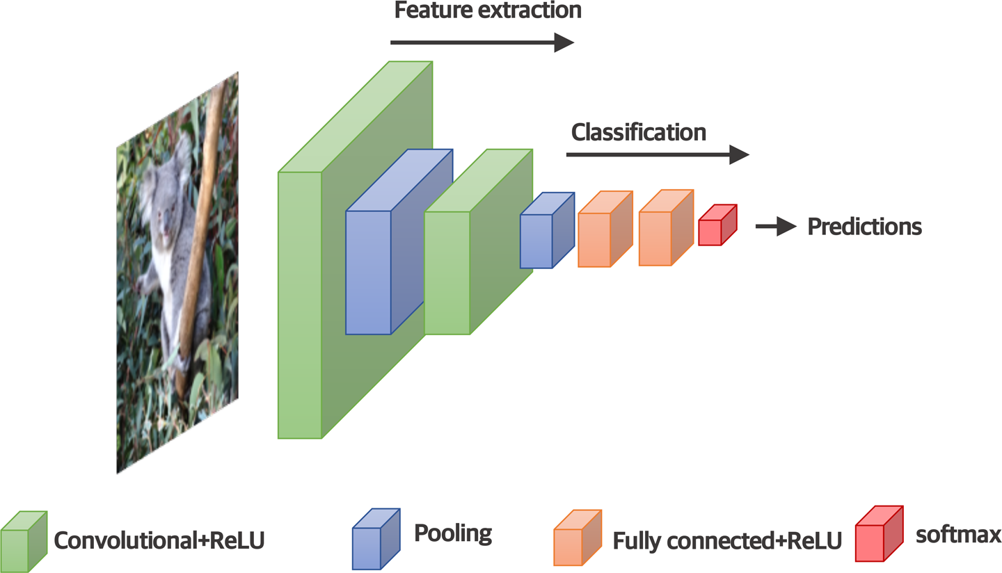
Figure 4-6. An example CNN image classification architecture
This batching is useful during training, when the model is being optimized for high volumes of training instances, and it also makes processing of multiple images simpler when the model is being tested and used operationally. Therefore, the dimensionality of an input tensor for a CNN will be four, not three. For example, if 50 color images of 224 x 224 pixels were passed to a neural network, the shape of this 4D input tensor would be:
shape=(50,224,224,3)
That’s 50 images, each of 224 x 224 pixels, and 3 color channels.
Most image processing neural networks take advantage of convolutional layers, so are classified as CNNs. However, their architectures vary considerably. In fact, one of the interesting challenges in DNN processing over recent years has been to create new architectures that are more accurate, learn faster, or take up less storage. There have been many approaches for image processing, as described in the following note.
Audio
Sound is our ears’ interpretation of pressure waves generated in the environment by anything that causes the air to vibrate. As with any waveforms, sound waves can be characterized by their amplitude and frequency.
The amplitude of the wave represents the variation in pressure and relates to our perception of the loudness of any noise. As with light, the frequency of the wave is the inverse of the wavelength, measured in Hertz (Hz). Shorter sound waves have higher frequencies and higher pitch. Longer sound waves have lower frequencies and lower pitch. Humans typically are able to hear waves ranging from 20 Hz to 20,000 Hz, and this is what we might classify as “sound.” However, for other animals or for digital sensors, this range might be quite different.
The simple characterization of amplitude and frequency fails to grasp the full complexity of sounds. To understand why, take a look at the sound waves in Figure 4-7. Sound wave a and sound wave b are clearly very different, but they have the exact same amplitude and fundamental frequency.
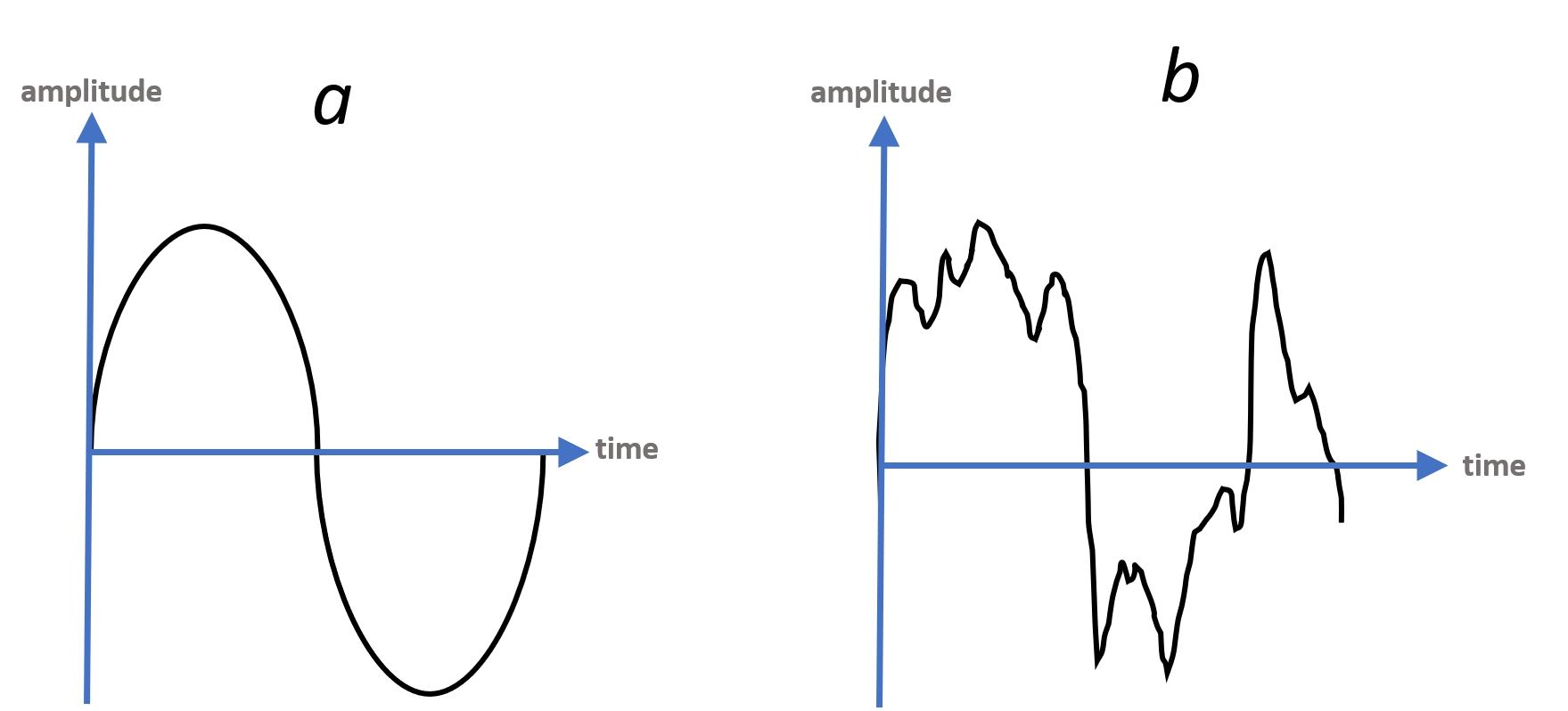
Figure 4-7. Two very different sound waves sharing the same wavelength (frequency) and amplitude
Sound wave a illustrates what we might consider a “perfect” simple sound wave representing a single tone. Sound wave b, however, is indicative of the messy sound that we hear day-to-day—that is, a wave derived from multiple frequencies from varying sources that bounce off objects and combine into complicated harmonics.
Digital Representation of Audio
Analog sound waves are transformed to digital format by capturing the intensity of the wave at regular sampling intervals. The simplest representation of a digital audio signal is therefore a list of numbers, where each number depicts the intensity of the sound wave at a specific time.
Once again, let’s think about precision as this will be important to an adversary in generating adversarial audio. Precision of digital audio depends upon two things: the rate at which the samples are taken and the accuracy of each intensity value. This is measured in terms of the frequency at which the analog data was sampled and the accuracy with which each sample is encoded—the sample rate and number of bits per sample (or “bit depth”), respectively. The bit depth determines the accuracy with which each sound sample is captured, akin to color resolution in image data. The sampling rate is the audio temporal equivalent to image spatial resolution. This is illustrated in Figure 4-8.
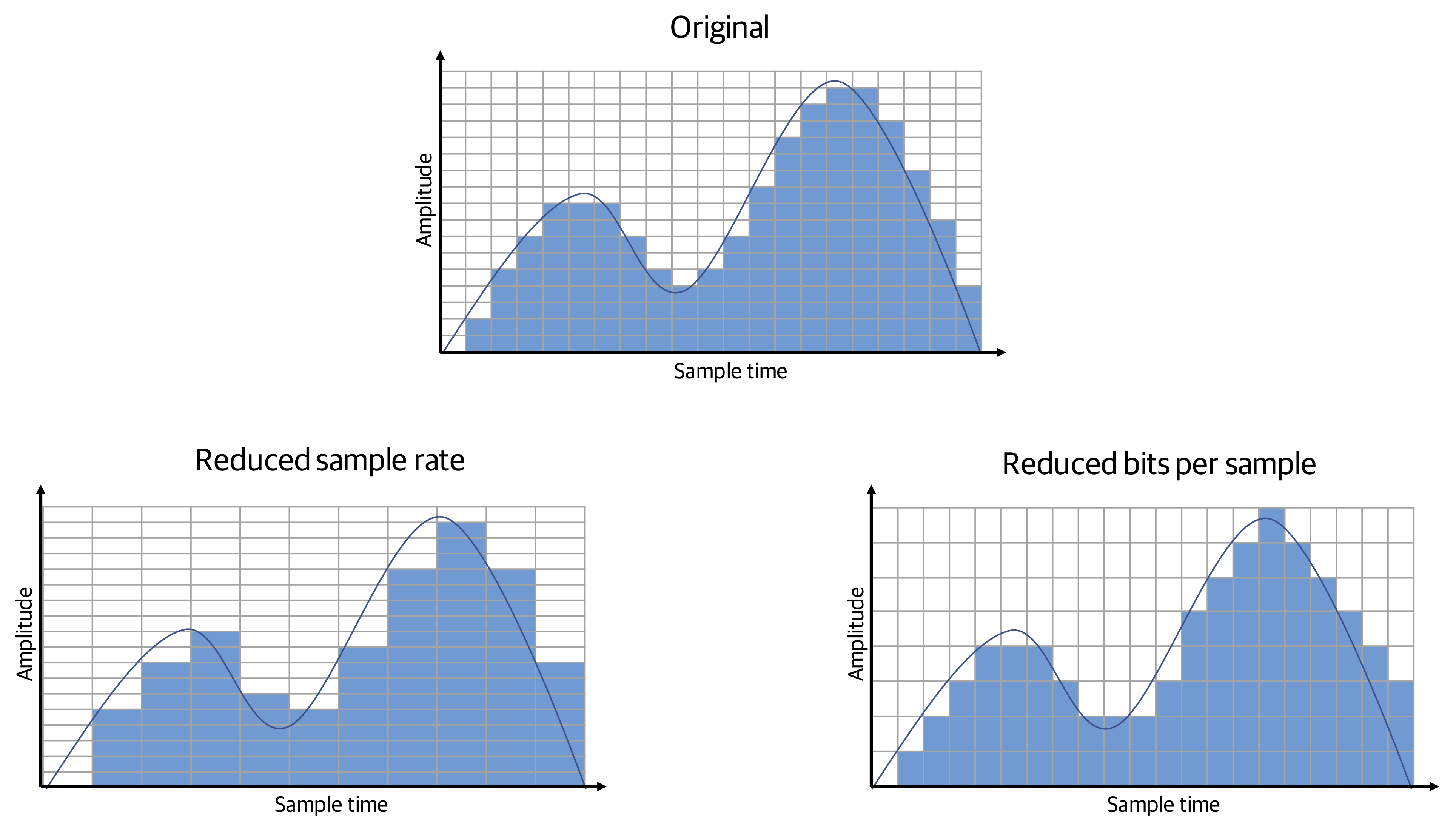
Figure 4-8. The effect of reduced sample rate and bits per sample in digital audio
DNNs for Audio Processing
As with image processing, audio processing existed for many years prior to the prevalence of DNN technology. DNNs remove the requirement to handcraft the features of the audio. However, audio processing using neural networks still often exploits traditional methods to extract low-level feature information common to all tasks.
Very broadly speaking, we might adopt one of two approaches to processing audio data using neural network technology:
-
First, we could train the data using the raw digitally encoded audio. The network would then learn to extract the features relevant to its task. This can produce highly accurate models, but the amount of data required for the network to learn from raw, messy audio is vast, so this approach is often not feasible.
-
Alternatively, we can give the neural network a head start by exploiting more traditional audio preprocessing steps, then using the preprocessed data to train the network. Preprocessing has the advantage that it reduces the amount of learning required by the network, thereby simplifying the training step and reducing the amount of data required for training.
Audio preprocessing usually uses a Fourier transform, which is a really neat mathematical calculation to convert the complicated waveforms that represent many frequencies (as shown earlier in this chapter in Figure 4-7, image b) into their constituent frequency parts. This information can then be turned into a spectrogram, representing frequencies as they change over time.
To create a spectrogram, the amplitude of each frequency is calculated within consecutive (and possibly overlapping) time windows using a Fourier transform. To create a visual depiction of a spectrogram, these intensities can be represented using color and the frequency time windows concatenated to produce something like the images in Figure 4-9. The image on the left illustrates the concept; the one on the right is a real spectrogram.
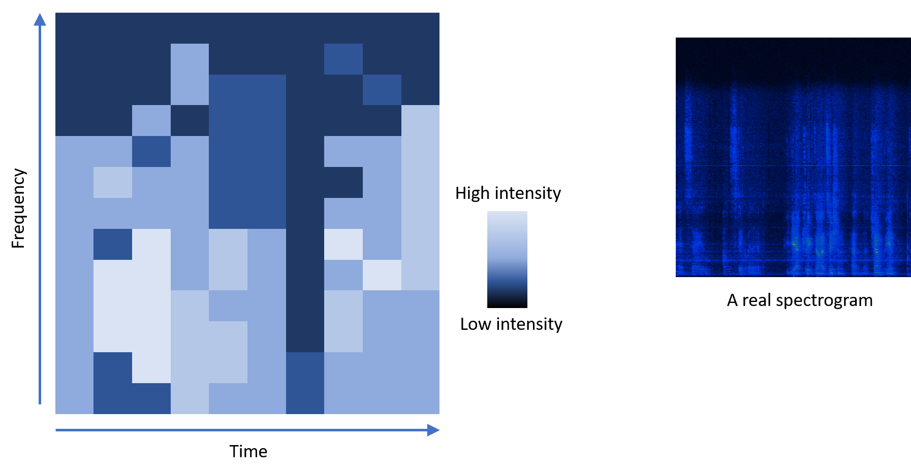
Figure 4-9. A spectrogram depicts changing intensities at different frequencies over time
In some cases, the preprocessing step may also extract only aspects of the audio that are pertinent to the task and discard other information. For example, audio may be transformed to mel-frequency cepstrum (MFC) representation to more closely represent the way in which audio data is treated in the human auditory system. This is particularly useful in processing that mimics human comprehension, such as speech processing.
Let’s consider a fundamental task in audio processing—classification. This is required as a precursor to other, more complex tasks such a speech processing. As in image classification, the task is to assign an audio clip to a classification based on the audio characteristics. The set of possible classifications will depend upon the test data and the application, but could be, for example, identifying a particular birdsong or a type of sound, such as “engine.”
So, how could we do this using a DNN? One method is to repurpose the CNN architecture by simply taking the spectrogram image and essentially turning the problem into one of image processing. The visual features within the spectrogram will be indicative of the audio that produced it, so, for example, a barking dog sound might have visual features that a CNN architecture would extract. This solution is essentially converting the time dimension into a spatial one for processing by the network.
Alternatively, a different type of neural network capable of dealing with sequences could be used. This type of network is called a recurrent neural network.
Introducing RNNs
RNNs are able to learn patterns and correlations in sequential data by processing each piece of data in the context of what has been processed before it and what comes afterward. Examples of data with meaning determined by sequence are text and time-based information such as speech. Patterns across sequences of data are not going to be detected by a simple feed-forward DNN or CNN because they only consider a single input in isolation. RNNs, however, are able to find correlations or patterns in sequential data by maintaining some kind of memory (or state) between inputs.
The simplest architectural approach for an RNN is for a hidden layer to take its input not only from the previous layer but also from its own output. Put another way, the output from the layer is fed forward to the next layer (as we have seen previously) but also fed back into itself, providing some input to the current layer’s calculation. This allows the hidden layer’s previous output to contribute to the processing of the current input. Figure 4-10 shows a simple illustration of this.
A challenge facing simple RNNs is that they are unable to learn patterns that span across longer sequences; that is, correlations that are separated by other data in the sequence. A good example of this is speech, where the likelihood of a particular phoneme might depend upon the sounds heard a few moments previously. During training of these simple RNNs, the cost function gradients have a tendency to vanish or become infinite. Essentially, the mathematical optimization step isn’t able to reach a good solution that accounts for these longer-spaced sequential relationships. This makes it impossible to adequately minimize the cost function so that the RNN performs well.
A more complex type of RNN called a long short-term memory (LSTM) network is commonly used to address this problem. The RNN nodes within an LSTM are far more complex units than shown in Figure 4-10, comprising a component that retains state and regulators (called “gates”) that control the data flow. This more complex architecture enables the network to both “remember” previous data in the sequence and “forget” previous data that is deemed less important. It’s this ability to forget that makes optimizing the network during training possible.
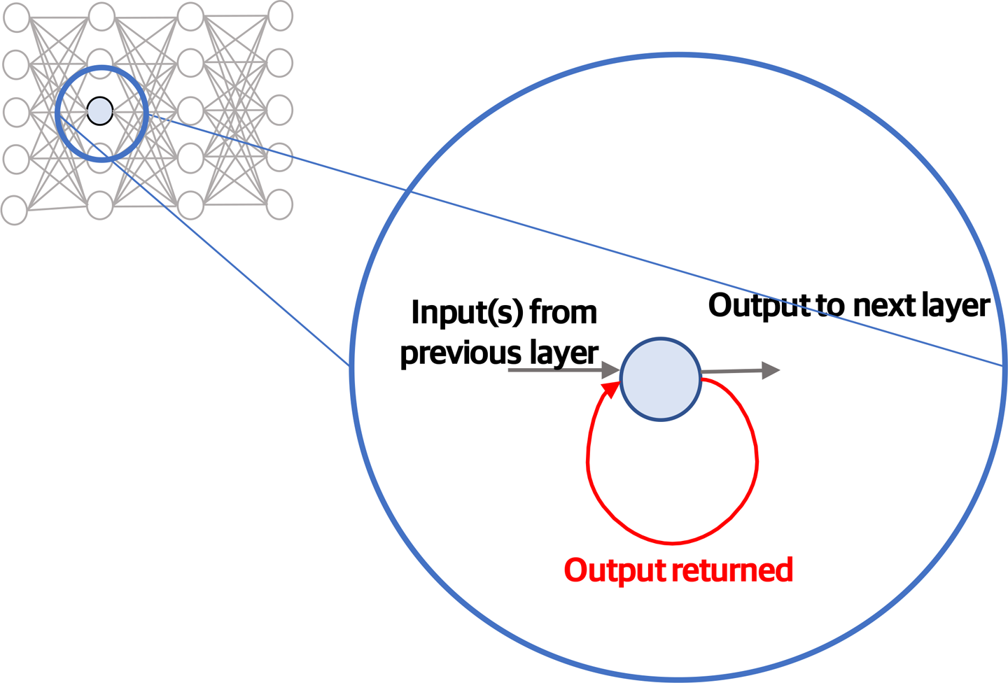
Figure 4-10. Basic concept underpinning RNN architectures
The various types of LSTMs have slightly different LSTM unit designs (for example, different gates). LSTMs have proven very effective across several applications, such as handwriting and speech recognition.
LSTMs are a common architectural choice for audio processing to enable the network to learn audio patterns that span time. This is obviously very applicable to understanding audio where the meaning of its parts depends on what is on either side (such as birdsong or speech). As an example, Figure 4-11 depicts the use of an RNN in processing audio that has been previously converted into a spectrogram. The preprocessed frequency information is a 2D tensor (a 2D matrix) representing the amplitude of each frequency in one dimension and time in the other.5 In this example, the same number of frames are output from the RNN, each one corresponding to the output of the RNN for a particular input in the sequence—one set of sound frequencies for a particular time generates a set of probabilities of possible sounds.

Figure 4-11. Typical processing chain for audio, with spectrogram preprocessing
Speech Processing
Speech processing is a fascinating application of DNNs which has considerable relevance to adversarial audio—many motivations for generating adversarial sound are likely for fooling speech recognition systems.
Speech recognition is a particularly challenging computational task. First, there’s the extraction of the sounds that form the building blocks of speech, known as phonemes. People are sloppy with their speech, they have different accents, they speak at different speeds and pitches, and there’s often background noise. All of this makes correct identification of each individual phoneme difficult. The extracted phonemes must then be mapped to real words and sentences. There may be many possible mappings; the correct mapping will depend on the language and the context.
In speech-to-text processing, the neural network is typically a part of a bigger processing chain. For example, a typical speech-to-text processing chain might look something like this:
-
An LSTM takes an audio MFC spectrogram as input and produces a list of the current probabilities for each of the possible symbols in a text system. This is the step depicted in Figure 4-11. In English, the probabilities would refer to the probabilities of each of the letters “a” to “z” and the “word space” character.6
-
The probability distributions are output from the LSTM at the same rate as they are input. This is a big problem because someone could be speaking really sssslllloooowwwwlllllyyyyy, or they might speakreallyfast. So, the length of the probability sequence indicates the length of the input audio, rather than the length of a phonetic transcription. Working out the alignments of the audio input with the phonetic transcription is another step in the processing.
A commonly used approach is connectionist temporal classification (CTC).7 CTC essentially “squashes” and tidies up the symbol probabilities to create probable phrases. For example, CTC would take a high-probability output such as
_cc_aa_tand generatecat. -
At this stage, there’s a list of probabilities for different phonetic transcriptions but no decisive phrase. The final step requires taking the most probable “raw” phrases and mapping them to transcripts appropriate to the language. A lot of this stuff is not possible to learn through generalization (for example, many words in English do not map to their phonetic equivalents). Therefore, this part of the processing likely uses a “language model” that encodes information about the language, probability of sequences, spellings and grammar, and real names.
Video
Video is a combination of moving image and audio. For completeness, in this section we’ll have a brief look at moving images, as audio was covered previously.
DNNs for Video Processing
It’s possible to analyze video simply by considering each image in isolation, which may be perfectly adequate for many scenarios. For example, facial detection and recognition can be performed on a frame-by-frame basis by feeding each frame into the neural network one by one. However, the additional dimension of time opens opportunities for understanding movement. This allows video understanding to extend to more complex semantic understanding, such as:
- Entity tracking
-
Tracking the paths of specific objects (such as people or vehicles) over time. This might include inferring positional information when the entity is obscured or leaves the scene.
- Activity recognition
-
Extending the idea of object recognition to detect activities within a scene using additional information pertaining to movement. For example, this could be understanding gestures used to control a device or detecting behavior (such as aggression) within a scene. The ability to recognize activities within videos enables other higher-level processing, such as video description.
As with image and audio, there are more classical approaches to video processing that do not use neural networks. But, once again, DNNs remove the requirement to hand-code the rules for extracting features.
Unsurprisingly, the element of time will add complexity to processing frames. There are, however, approaches to dealing with this additional dimension using the architectural principles described previously for CNNs and RNNs. For example, one option is to exploit 3D Convolutions. This extension of the convolutional principles used in image CNNs includes a third temporal dimension across frames which is processed in the same way as spatial dimensions within each frame. Alternatively, it’s possible to combine spatial learning of a CNN with sequential learning borrowed from an RNN architecture. This can be done by exploiting the CNN to extract features on a per-frame basis and then using these features as sequential inputs to an RNN.
Whereas color images are passed to a neural network as a 4D tensor, video inputs are represented by a whopping 5D tensor. For example, if we have one minute’s worth of video sampled at 15 frames per second, that gives us 900 frames. Let’s assume low-definition video (224 x 224 pixels) and color using RGB channels. We have a 4D tensor with the following shape:
shape=(900,224,224,3)
If there are 10 videos in the input batch, the shape becomes 5D:
shape=(10,900,224,224,3)
Adversarial Considerations
This chapter provided an introduction to the variety of neural networks available, with a focus on those commonly used for image, audio, and video processing. Some aspects of these neural networks are defined by the software developer, whereas others are learned during training. Aspects defined by the developer are defined as the model architecture and the learned parts of the model as the model parameters. It’s not important to understand the details of specific DNN architectures and parameters in order to acquire a good conceptual understanding of adversarial examples. However, it is good to appreciate the difference between a model’s architecture and its learned parameters because an understanding of the target network architecture and its parameters can be important when generating adversarial examples:
- Model architecture
-
At the highest level, the model architecture is the types of layers in the model and the order in which they are placed. The model architecture also defines the predetermined aspects of the configuration of the model. In the code at the end of Chapter 3, we defined the number of layers, the types of layers (ReLU and softmax), and the size of each layer. More complex layers, such as CNN layers, introduce more architectural decisions, such as the size and number of filters in a convolutional layer, the type of pooling, and the pooling window size plus the convolving step movement (the “stride”) for each of the pooling and convolutional steps.
- Model parameters
-
In terms of model parameters, most obvious are the values of the weights and biases, as learned during the training phase in the example in Chapter 3. There are often many other parameters that also must be learned in more complex layers, such as the values that make up each convolutional filter.
While there are not “set” architectures for any particular task, there are certainly reusable architectural patterns, such as convolutional layers or LSTM units.
Adversarial input has primarily been researched in the context of image classification and (to a lesser extent) speech recognition, but other similar types of tasks will also be susceptible to this trickery. For example, while most interest in adversarial imagery has related to fooling image classifiers, the adversarial techniques are also likely applicable to object detection and localization and semantic segmentation, as they are essentially extensions of the more basic classification task.8 Facial recognition is another example—creating adversarial input to fool a facial recognition system does not, in principle, differ from creating adversarial images for misclassification of other objects. However, there may be other complexities; for example, the adversarial changes may be more difficult to hide on a face. In the audio domain, adversarial examples have been proven for speech recognition, but the same methods could also be applied to simpler tasks (such as voice verification and more generic audio classification).
Image Classification Using ResNet50
To illustrate image classification, the examples in this book use ResNet50, rather than one of the other models available online. It’s a fairly arbitrary decision based primarily on the fact that the model doesn’t require much space (approximately 102 MB). All the other current state-of-the-art image classification neural networks have also been proven to be vulnerable to adversarial input.
This section demonstrates how to download the ResNet50 classifier and generate predictions for one or more images. Later, this will be useful for testing adversarial examples.
Note
You can find the code snippets in the Jupyter notebook chapter04/resnet50_classifier.ipynb on the book’s GitHub repository.
We begin by importing the TensorFlow and Keras libraries and the ResNet50 model:
importtensorflowastffromtensorflowimportkerasfromkeras.applications.resnet50importResNet50importnumpyasnpmodel=ResNet50(weights='imagenet',include_top=True)

We will use NumPy to manipulate the image data as a multidimensional array.

This command instantiates the ResNet50 model that has been trained on ImageNet.
include_top=Trueindicates that the final neural network layers that perform the classification should be included. This option is provided because these classification layers may not be required if the purpose of the model is to extract the relevant features only.
As with the Fashion-MNIST classifier, it’s nice to see what the model looks like:
model.summary()
This generates the following output (the depth of ResNet50 makes the output from this call very lengthy, so only the initial and final layers are captured here):
_________________________________________________________________________________
Layer (type)                   Output Shape         Param #  Connected to
=================================================================================
input_1 (InputLayer)           (None, 224, 224, 3)  0
_________________________________________________________________________________
conv1_pad (ZeroPadding2D)      (None, 230, 230, 3)  0        input_1[0][0]
_________________________________________________________________________________
conv1 (Conv2D)                 (None, 112, 112, 64) 9472     conv1_pad[0][0]
_________________________________________________________________________________
bn_conv1 (BatchNormalization)  (None, 112, 112, 64) 256      conv1[0][0]
_________________________________________________________________________________
activation_1 (Activation)      (None, 112, 112, 64) 0        bn_conv1[0][0]
_________________________________________________________________________________
pool1_pad (ZeroPadding2D)      (None, 114, 114, 64) 0        activation_1[0][0]
_________________________________________________________________________________
max_pooling2d_1 (MaxPooling2D) (None, 56, 56, 64)   0        pool1_pad[0][0]
_________________________________________________________________________________

...

_________________________________________________________________________________
activation_49 (Activation)     (None, 7, 7, 2048)   0        add_16[0][0]
_________________________________________________________________________________
avg_pool (GlobalAveragePooling2(None, 2048)         0        activation_49[0][0]
_________________________________________________________________________________
fc1000 (Dense)                 (None, 1000)         2049000  avg_pool[0][0]
=================================================================================
Total params: 25,636,712
Trainable params: 25,583,592
Non-trainable params: 53,120
Let’s get an image to classify (Figure 4-12):
importmatplotlib.pyplotaspltimg_path='../images/koala.jpg'img=image_from_file(img_path,(224,224))plt.imshow(img)
You’ll find a selection of images in the repository, but of course you can try your own as well.
image_from_fileis a simple helper utility to open an image and scale it to 244 x 244 pixels for input to the classifier. For brevity, this function is not included here, but it is included as a Python utility in the GitHub repository.
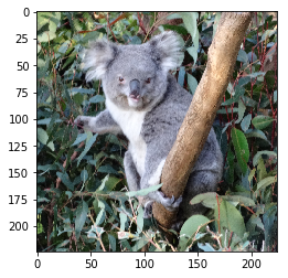
Figure 4-12. Code output
The image needs to undergo some preprocessing before it is passed to ResNet50. Keras provides the preprocessing function (preprocess_input):
fromkeras.applications.resnet50importpreprocess_inputnormalized_image=preprocess_input(img)
This preprocessing step prepares the image so that it is in the same
format as the images that were used to train the network. This will depend upon the model being used. For ResNet50, preprocess_input transforms the image in the following ways:
- Normalization
-
Subtracting the mean RGB values for the complete training data centers data around the zero mean for each of the channels. Normalizing the training data in this way helps the network to learn faster. Subsequent test data passed to the network should undergo the same normalization.
- Switching channel order
-
ResNet50 was trained on images with the channels ordered as BGR, rather than RGB. If the image is in RGB format, the channel order needs to be switched.
Note
To see the preprocessing steps in detail, visit the Jupyter notebook chapter04/resnet50_preprocessing.ipynb on this book’s GitHub site.
The normalized image can now be passed to the classifier:
normalized_image_batch=np.expand_dims(normalized_image,0)predictions=model.predict(normalized_image_list)
The classifier takes a batch of images in the form of
np.arrays, soexpand_dimsis required to add an axis to the image. This makes it a batch containing one image.
We now have the predictions that are the vector output from the final layer of the classifier—a big array representing the probabilities for every classification. The top three classifications along with their predictions can be printed out nicely using the following code:
fromkeras.applications.resnet50importdecode_predictionsdecoded_predictions=decode_predictions(predictions,top=3)predictions_for_image=decoded_predictions[0]forpredinpredictions_for_image:(pred[1],':',pred[2])
decode_predictionsis a handy helper utility to extract the highest predictions in thepredictionsarray (in this case the top three) and associate them with their associated labels.
Here’s the output:
koala  :  0.999985
indri  :  7.1616164e-06
wombat  :  3.9483125e-06
Superb classification by ResNet50! In the next part of this book, we’ll see how the model, when presented with the same image with very minor perturbation, will do considerably worse.
1 This image was generated using SegNet.
2 K. Simonyan and A. Zisserman, “Very Deep Convolutional Networks for Large-Scale Image Recognition,” ImageNet Large Scale Visual Recognition Challenge (2014), http://bit.ly/2IupnYt.
3 K. He et al. “Deep Residual Learning for Image Recognition,” ImageNet Large Scale Visual Recognition Challenge (2015), http://bit.ly/2x40Bb6.
4 Christian Szegedy et al., “Going Deeper with Convolutions,” ImageNet Large Scale Visual Recognition Challenge (2014), http://bit.ly/2Xp4PIU.
5 This assumes a single audio channel. If the audio contains multiple channels, there is a third dimension representing the channel depth.
6 There’s also a special blank character, different from the space, to represent a gap in the audio.
7 A. Graves et al., “Connectionist Temporal Classification: Labelling Unsegmented Sequence Data with Recurrent Neural Networks,” Proceedings of the 23rd International Conference on Machine Learning (2006): 369–376, http://bit.ly/2XUC2sU.
8 This is demonstrated in Cihang Xie et al., “Adversarial Examples for Semantic Segmentation and Object Detection,” International Conference on Computer Vision (2017), http://bit.ly/2KrRg5E.
Get Strengthening Deep Neural Networks now with the O’Reilly learning platform.
O’Reilly members experience books, live events, courses curated by job role, and more from O’Reilly and nearly 200 top publishers.

