Python and R for the Modern Data Scientist

Chapter 4. Data Format Context

Boyan Angelov

In this chapter we’ll review tools in Python and R for importing and processing data in a variety of formats. We’ll cover a selection of packages, compare and contrast them, and highlight the properties that make them effective. At the end of this tour, you’ll be able to select packages with confidence. Each section illustrates the tool’s capabilities with a specific mini case study, based on tasks that a data scientist encounters daily. If you’re transitioning your work from one language to another or simply want to find out how to get started quickly using complete, well-maintained, and context-specific packages, this chapter will guide you.

Before we dive in, remember that the open source ecosystem is constantly changing. New developments, such as transformer models and explainable artificial intelligence (XAI), seem to emerge every other week. These often aim at lowering the learning curve and increasing developer productivity. This explosion of diversity also applies to related packages, resulting in a nearly constant flow of new and (hopefully) better tools. If you have a very specific problem, there’s probably a package already available for you, so you don’t have to reinvent the wheel. Tool selection can be overwhelming, but at the same time this variety of options can improve the quality and speed of your data science work.

The package selection in this chapter can appear limited in view; hence, it is essential to clarify our selection criteria. So what qualities should we look for in a good tool?

It should be open source.

There is a large number of valuable commercial tools available, but we firmly believe that open source tools have a great advantage. They tend to be easier to extend and understand what their inner workings are, and are more popular.

It should be feature-complete.

The package should include a comprehensive set of functions that help the user do their fundamental work without resorting to other tools.

It should be well maintained.

One of the drawbacks of using open source software (OSS) is that sometimes packages have a short life cycle, and their maintenance is abandoned (so-called “abandonware”). We want to use packages that are actively worked on so we can feel confident they are up-to-date.

Let’s begin with a definition. What is a data format? There are several answers available. Possible candidates are data type, recording format, and file format. Data type is related to data stored in databases or types in programming languages (for example integer, float, or string). The recording format is how data is stored in a physical medium, such as a CD or DVD. And finally, what we’re after, the file format, i.e., how information is prepared for a computing purpose.

With that definition in hand, you might still wonder why I dedicate an entire chapter to focus just on file formats. You have probably been exposed to them in another context, such as saving a PowerPoint slide deck with a .ppt or .pptx extension (and wondering which one is better). The problem here goes much further beyond basic tool compatibility. The way information is stored influences the complete downstream data science process. For example, if our end goal is to perform advanced analytics and the information is stored in a text format, we have to pay attention to factors such as character encoding (a notorious problem, especially for Python).¹ For such data to be effectively processed, it also needs to go through several steps, such as tokenization and stop word removal.² Those same steps are not applicable to image data, even though we may have the same end goal in mind, e.g., classification. In that case other processing techniques are more suitable, such as resizing and scaling. These differences in data processing pipelines are shown in Figure 4-1. To summarize: the data format is the most significant factor influencing what you can and cannot do with it.

Note

We now use the word pipeline for the first time in this context, so let’s use the opportunity to define it. You have probably heard the expression that “data is the new oil.” This expression goes beyond a simple marketing strategy and represents a useful way to think about data. There are surprisingly many parallels between how oil and data are processed. You can imagine that the initial data that the business collects is the rawest form—probably of limited use initially. It then undergoes a sequence of steps, called data processing, before it’s used in some application (i.e., for training an ML model or feeding a dashboard). In oil processing, this would be called refinement and enrichment—making the data usable for a business purpose. Pipelines transport the different oil types (raw, refined) through the system to its final state. The same term can be used in data science and engineering to describe the infrastructure and technology required to process and deliver data.

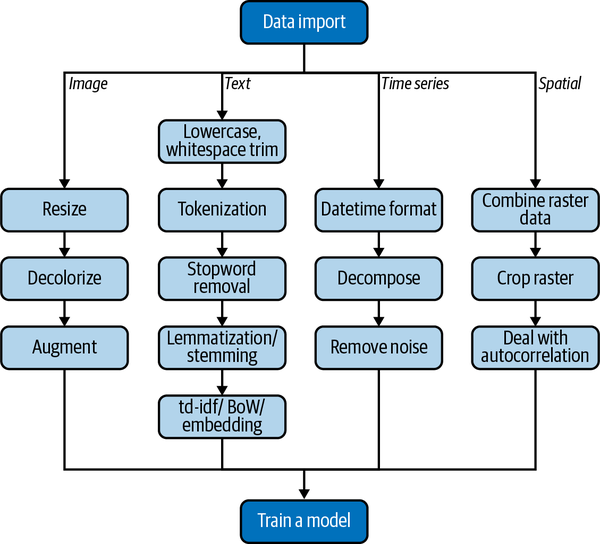
Figure 4-1. Difference between common data format pipelines (the lighter shade indicates the shared steps between the workflows)

Infrastructure and performance also need to be taken into consideration when working with a specific data format. For example, with image data, you’ll need more storage availability. For time-series data you might need to use a particular database, such as InfluxDB. And finally, in terms of performance, image classification is often solved using deep learning methods based on convolutional neural networks (CNNs), which may require a graphics processing unit (GPU). Without it, model training can be very slow and become a bottleneck both for your development work and a potential production deployment.

Now that we have covered the reasons to carefully consider which packages to use, we’ll have a look at the possible data formats. This overview is presented in Table 4-1 (note that those tools are mainly designed for small- to medium-size datasets). Admittedly, we are just scratching the surface on what’s out there, and there are a few notable omissions (such as audio and video). Here, we’ll focus on the most widely used formats.

Table 4-1. An overview of data formats and popular Python and R packages used to process data stored in them

Data type	Python package	R package
Tabular	pandas	readr, rio
Image	open-cv, scikit-image, PIL	magickr, imager, EBImage
Text	nltk, spaCy	tidytext, stringr
Time series	prophet, sktime	prophet, ts, zoo
Spatial	gdal, geopandas, pysal	rgdal, sp, sf, raster

This table is by no means exhaustive, and we are certain new tools will appear soon, but these are the workhorses fulfilling our selection criteria. Let’s get them to work in the following sections, and see which ones are the best for the job!

External Versus Base Packages

In Chapter 2 and Chapter 3, we introduced packages very early in the learning process. In Python we used pandas right at the outset and transitioned to the Tidyverse in R relatively quickly. This allowed us to be productive much faster than if we went down the rabbit holes of archaic language features that you’re unlikely to need as a beginner.³ A programming language’s utility is defined by the availability and quality of its third-party packages, as opposed to the core features of the language itself.

This is not to say that there aren’t a lot of things that you can accomplish with just base R (as you’ll see in some of the upcoming examples), but taking advantage of the open source ecosystem is a fundamental skill to increase your productivity and avoid reinventing the wheel.

Go Back and Learn the Basics

There is a danger in overusing third-party packages, and you have to be aware of when the right time to go back to the basics is. Otherwise you might fall victim to a false sense of security and become reliant on the training wheels provided by tools such as pandas. This might lead to difficulties when dealing with more specific real-world challenges.

Let’s now see how this package versus base language concept plays out in practice by going into detail with a topic we’re already familiar with: tabular data.⁴ There are at least two ways to do this in Python. First, using pandas:

import pandas as pd

data = pd.read_csv(“dataset.csv”)

Second, with the built-in csv module:

import csv

with open(“dataset.csv”, “r”) as file: 
	reader = csv.reader(file, delimiter=“,”)
for row in reader: 
	print(row)

Note how you need to specify the file mode, in this case "r" (standing for “read”). This is to make sure the file is not overwritten by accident, hinting at a more general-purpose oriented language.

Using a loop to read a file might seem strange to a beginner, but it makes the process explicit.

This example tells us that pd.read_csv() in pandas provides a more concise, convenient, and intuitive way to import data. It is also less explicit than vanilla Python and not essential. pd.read_csv() is, in essence, a convenience wrapper of existing functionality—good for us!

Here we see that packages serve two functions. First, as we have come to expect, they provide new functionality. Second, they are also convenience wrappers for existing standard functions, which make our lives easier.

This is brilliantly demonstrated in R’s rio package.⁵ rio stands for “R input/output,” and it does just what it says.⁶ Here, the single function import() uses the file’s filename extension to select the best function in a collection of packages for importing. This works in Excel, SPSS, stata, SAS, and many other common formats.

Another R Tidyverse package called vroom allows for fast import of tabular data and can read an entire directory of files in one command, with the use of map() functions or for loops.

Finally, the data.table package, which is often neglected at the expense of promoting the Tidyverse, provides the exceptional fread(), which can import very large files at a fraction of what base R or readr offer.

The usefulness of learning how to use third-party packages becomes more apparent when we try to perform more complex tasks, as we’ll see next when processing other data formats.

Data Science from Scratch

Writing software from scratch is a great way to understand how things work under the hood. It’s a recommended step in learning, especially after getting used to the tools at higher abstraction levels (such as scikit-learn). Excellent reading material on this topic is provided in Joel Grus’s book Data Science from Scratch (O’Reilly, 2019).

Now that we can appreciate the advantages of packages, we’ll demonstrate some of their capabilities. For this we’ll work on several different real-world use cases, listed in Table 4-2. We won’t focus on minute implementation details, but instead cover the elements that expose their benefits (and shortcomings) for the tasks at hand. Since the focus in this chapter is on data formats, and Chapter 5 is all about workflows, all these case studies are about data processing.

Note

For pedagogic purposes we have omitted parts of the code. If you’d like to follow along, executable code is available in the book’s repository.

Table 4-2. An overview of the different use cases

Data format	Use case
image	Swimming pool and car detection
text	Amazon product reviews processing
time series	Daily Australian temperatures
spatial	Loxodonta africana species distribution data

Further information on how to download and process these data is available in the official repository for the book.

Image Data

Images pose a unique set of challenges for data scientists. We’ll demonstrate the optimal methodology by covering the challenge of aerial image processing—a domain of growing importance in agriculture, biodiversity conservation, urban planning, and climate change research. Our mini use case utilizes data from Kaggle collected to help the detection of swimming pools and cars. For more information on the dataset, you can use the URL in Table 4-2.

As we mentioned at the beginning of the chapter, downstream purpose influences data processing heavily. Since aerial data is often used to train machine learning algorithms, our focus will be on preparatory tasks.

The OpenCV package is one of the most common ways to work with image data in Python. It contains all the necessary tools for image loading, manipulation, and storage. The “CV” in the name stands for computer vision—the field of machine learning that focuses on image data. Another handy tool that we’ll use is scikit-image. As its name suggests, it’s very much related to scikit-learn.⁷

Here are the steps of our task (refer to Table 4-2):

1. Resize the image to a specific size.

2. Convert the image to black and white.

3. Augment the data by rotating the image.

For an ML algorithm to learn successfully from data, the input has to be cleaned (data munging), standardized (scaling), and filtered (feature engineering).⁸ You can imagine gathering a dataset of images (e.g., by scraping data from Google Images).⁹ They will differ in some way or another—such as size and/or color. Steps 1 and 2 in our task list help us deal with that. Step 3 is handy for ML applications. The performance (i.e., classification accuracy, or area under the curve [AUC]) of ML algorithms depends mostly on the amount of training data, which is often in little supply. To get around this, without resorting to obtaining more data,¹⁰ data scientists have discovered that playing around with the data already available, such as rotating and cropping, can introduce new data points. Those can then be used to train the model again and improve performance. This process is formally known as data augmentation.¹¹

Enough talk—let’s import the data! Check the complete code at the book’s repository if you want to follow along. The results are in Figure 4-2.

import cv2 
single_image = cv2.imread("img_01.jpg")

plt.imshow(single_image)
plt.show()

Using cv2 might seem confusing since the package is named OpenCV. cv2 is used as a shorthand name. The same naming pattern is used for scikit-image, where the import statement is shortened to skimage.

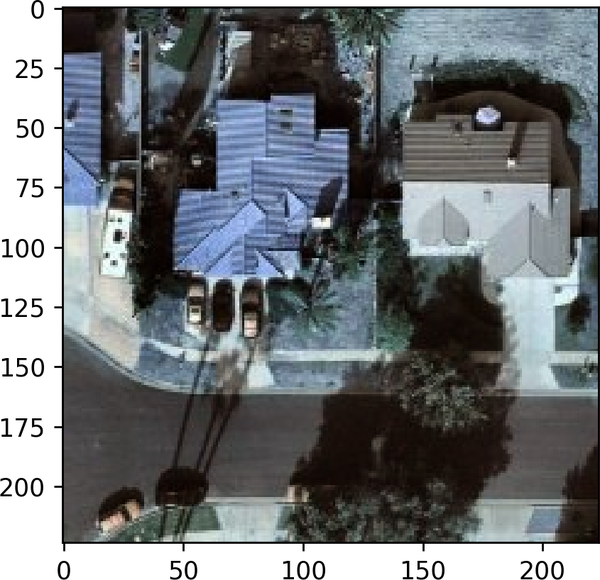
Figure 4-2. Raw image plot in Python with matplotlib

So in what object type did cv2 store the data? We can check with type:

print(type(single_image))
numpy.ndarray

Here we can observe an important feature that already provides advantages to using Python for CV tasks as opposed to R. The image is directly stored as a NumPy multidimensional array (nd stands for n-dimensions), making it accessible to a variety of other tools available in the wider Python ecosystem. Because this is built on the PyData stack, it’s well supported. Is this true for R? Let’s have a look at the magick package:

library(magick)
single_image <- image_read('img_01.jpg')
class(single_image)
[1] "magick-image"

The magick-image class is only accessible to functions from the magick package, or other closely related tools, but not the powerful base R methods (such as the ones shown in Chapter 2, with the notable exception of plot()). The differences in approaches of various open source packages supporting each other is illustrated in Figure 4-3, and is a common thread throughout the examples in this chapter.

Note

There is at least one exception to this rule—the EBImage package, a part of BioConductor. By using it you can get access to the image in its raw array form, and then use other tools on top of that. The drawback here is that it’s part of a domain-specific package, and it might not be easy to see how it works in a standard CV pipeline.

Note that in the previous step (where we loaded the raw image in Python), we also used one of the most popular plotting tools, matplotlib (data visualization is covered in Chapter 5), so we again took advantage of this better design pattern.

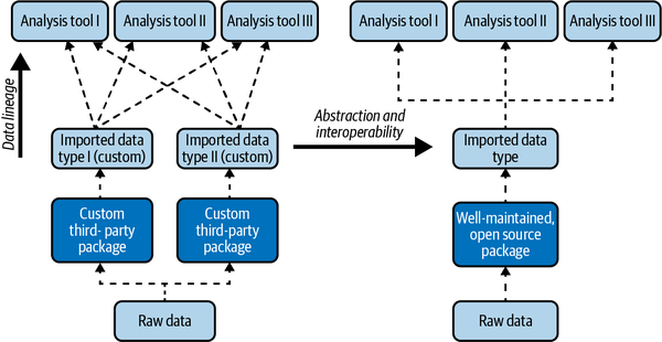
Figure 4-3. The two types of package design hierarchies as they are used during a data life cycle (bottom to top)

Now that we know that the image data is stored as a NumPy ndarray, we can use NumPy’s methods. What’s the size of the image? For this we can try the .shape method of ndarray:

print(single_image.shape)
224 224 3

It worked indeed! The first two output values correspond to the image height and width respectively, and the third one to the number of channels in the image—three in this case ((r)ed, (g)reen, and (b)lue). Now let’s continue and deliver on the first standardization step—image resizing. Here we’ll use cv2 for the first time:

single_image = cv2.resize(single_image,(150, 150))
print(single_image.shape)
(150, 150, 3)

Tip

If you gain experience working with such fundamental tools in both languages, you’ll be able to test your ideas quickly, even without knowing whether those methods exist. If the tools you use are designed well (as in the better design in Figure 4-3), often they will work as expected!

Perfect, it worked like a charm! The next step is to convert the image to black and white. For this, we’ll also use cv2:

gray_image = cv2.cvtColor(single_image, cv2.COLOR_RGB2GRAY)
print(gray_image.shape)
(150, 150)

The colors are greenish and not gray. This default option chooses a color scheme that makes the contrast more easily discernible for a human eye than black and white. When you look at the shape of the NumPy ndarray, you can see that the channel number has disappeared—there is just one now. Now let’s complete our task, do a simple data augmentation step, and flip the image horizontally. Here we’re again taking advantage that the data is stored as a NumPy array. We’ll use a function directly from NumPy, without relying on the other CV libraries (OpenCV or scikit-image):

flipped_image = np.fliplr(gray_image)

The results are shown in Figure 4-4.

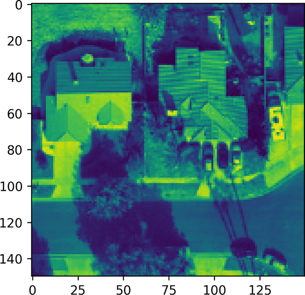
Figure 4-4. Plot of an image flipped by using NumPy functions

We can use scikit-image for further image manipulation tasks such as rotation, and even this different package will work as expected on our data format:

from skimage import transform
rotated_image = transform.rotate(single_image, angle=45)

The data standardization and augmentation steps we went through illustrate how the less complex package design (Figure 4-3) makes us more productive. We can drive the point home by showing a negative example for the third step, this time in R. For that, we’ll have to rely on the adimpro package:

library(adimpro)
rotate.image(single_image, angle = 90, compress=NULL)

Whenever we load yet another package, we are decreasing the quality, readability, and reusability of our code. This issue is primarily due to possible unknown bugs, a steeper learning curve, or a potential lack of consistent and thorough documentation for that third-party package. A quick check on the status of adimpro on CRAN reveals that the last time it was updated was in November 2019.¹² This is why using tools such as OpenCV, which work on image data by taking advantage of the PyData stack,¹³ is preferred.

A less complex, modular, and abstract enough package design goes a long way to make data scientists productive and happy in using their tools. They are then free to focus on actual work and not dealing with complex documentation or a multitude of abandonware packages. These considerations make Python the clear winner in importing and processing image data, but is this the case for the other formats?

Text Data

The analysis of text data is often used interchangeably with the term natural language processing (NLP). This, in turn, is a subfield of ML. Hence it’s not surprising to see that Python-based tools also dominate it. The inherently compute-intensive nature of working with text data is one good reason why that’s the case. Another one is that dealing with larger datasets can be a more significant challenge in R than in Python (this topic is covered further in Chapter 5).¹⁴ And it is a big data problem. The amount of text data has proliferated in recent years with the rise of services on the internet and social media giants such as Twitter and Facebook. Such organizations have also invested heavily in the technology and related open source tools, due to the fact that a large chunk of data available to them is in text format.

Similarly to the image data case, we’ll start by designing a standard NLP task. It should contain the most fundamental elements of an NLP pipeline. For a dataset, we selected texts from the Amazon product reviews dataset (Table 4-2), and we have to prepare it for an advanced analytics use case, such as text classification, sentiment analysis, or topic modeling. The steps needed for completion are the following:

1. Tokenize the data.

2. Remove stop words.

3. Tag the parts of speech (PoS).

We’ll also go through more advanced methods (such as word embeddings) in spaCy to demonstrate what the Python packages are capable of and, at the same time, provide a few R examples for comparison.

So what are the most common tools in Python? The most popular one is often referred to as the Swiss Army knife of NLP—the Natural Language Toolkit (NLTK).¹⁵ It contains a good selection of tools covering the whole pipeline. It also has excellent documentation and a relatively low learning curve for its API.

As a data scientist, one of the first steps in a project is to look at the raw data. Here’s one example review, along with its data type:

example_review = reviews["reviewText"].sample()
print(example_review)
print(type(example_review))

I just recently purchased her ''Paint The Sky With Stars''
 CD and was so impressed that I bought 3 of her previously
 released CD's and plan to buy all her music.  She is
 truely talented and her music is very unique with a
 combination of modern classical and pop with a hint of
 an Angelic tone. I still recommend you buy this CD. Anybody
  who has an appreciation for music will certainly enjoy her music.

str

This here is important—the data is stored in a fundamental data type in Python—str (string). Similar to the image data being stored as a multidimensional NumPy array, many other tools can have access to it. For example, suppose we were to use a tool that efficiently searches and replaces parts of a string, such as flashtext. In that case, we’d be able to use it here without formatting issues and the need to coerce the data type.¹⁶

Now we can take the first step in our mini case study—tokenization. It will split the reviews into components, such as words or sentences:

sentences = nltk.sent_tokenize(example_review)
print(sentences)

["I just recently purchased her ''Paint The Sky With Stars''
CD and was so impressed that I bought 3 of her
previously released CD's and plan to buy all her music.",
 'She is truely talented and her music is very unique with
  a combination of modern classical and pop with a hint of an Angelic tone.',
 'I still recommend you buy this CD.',
 'Anybody who has an appreciation for music will certainly enjoy her music.']

Easy enough! For illustration purposes, would it be that hard to attempt this relatively simple task in R, with some functions from tidytext?

tidy_reviews <- amazon_reviews %>%
  unnest_tokens(word, reviewText) %>%
  mutate(word = lemmatize_strings(word, dictionary = lexicon::hash_lemmas))

This is one of the most well-documented methods to use. One issue with this is that it relies heavily on the “tidy data” concept, and also on the pipeline chaining concept from dplyr (we covered both in Chapter 2). These concepts are specific to R, and to use tidytext successfully, you would have to learn them first, instead of directly jumping to processing your data. The second issue is the output of this procedure—a new data.frame containing the data in a processed column. Although this might be what we need in the end, this skips a few intermediate steps and is several layers of abstraction higher than what we did with nltk. Lowering this abstraction and working in a more modular fashion (such as processing a single text field first) adheres to software development best practices, such as DRY (“Do not repeat yourself”) and separation of concerns.

The second step of our small NLP data processing pipeline is removing stop words:¹⁷

tidy_reviews <- tidy_reviews %>%
  anti_join(stop_words)

This code suffers from the same issues, along with a new confusing function—anti_join. Let’s compare it to the simple list comprehension (more information on this in Chapter 3) step in nltk:

english_stop_words = set(stopwords.words("english"))
cleaned_words = [word for word in words if word not in english_stop_words]

english_stop_words is just a list, and then the only thing we do is loop through every word in another list (words) and remove it if it’s present in both. This is easier to understand. There’s no relying on advanced concepts or functions that are not directly related. This code is also at the right level of abstraction. Small code chunks can be used more flexibly as parts of a larger text processing pipeline function. A similar meta processing function in R can become bloated—slow to execute and hard to read.

While nltk allows for such fundamental tasks, we’ll now have a look at a more advanced package—spaCy. We’ll use this for the third and final step in our case study—part of speech (PoS) tagging:¹⁸

import spacy

nlp = spacy.load("en_core_web_sm") 

doc = nlp(example_review) 
print(type(doc))

spacy.tokens.doc.Doc

Here we are loading all the advanced functionality we need through one function.

We take one example review and feed it to a spaCy model, resulting in the spacy.tokens.doc.Doc type, not a str. This object can then be used for all kinds of other operations:

for token in doc:
    print(token.text, token.pos_)

The data is already tokenized on loading. Not only that—all the PoS tags are marked already!

The data processing steps that we covered are relatively basic. How about some newer and more advanced NLP methods? We can take word embeddings, for example. This is one of the more advanced text vectorization methods,¹⁹ where each vector represents the meaning of a word based on its context. For that, we can already use the same nlp object from the spaCy code:

for token in doc:
    print(token.text, token.has_vector, token.vector_norm, token.is_oov)

for token in doc:...
I True 21.885008 True
just True 22.404057 True
recently True 23.668447 True
purchased True 23.86188 True
her True 21.763712 True
' True 18.825636 True

It’s a welcome surprise to see that those abilities are already built-in into one of the most popular Python NLP packages. On this level of NLP methods, we can see that there’s almost no alternative available in R (or even other languages, for that matter). Many analogous solutions in R rely on wrapper code around a Python backend (which can defeat the purpose of using the R language).²⁰ This pattern is often seen in the book, especially in Chapter 5. The same is also true for some other advanced methods such as transformer models.²¹

For Round 2, Python is again the winner. The capabilities of nltk, spaCy, and other associated packages make it an excellent choice for NLP work!

Time Series Data

The time-series format is used to store any data with an associated temporal dimension. It could be as simple as shampoo sales from a local grocery store, with a timestamp, or millions of data points from a sensor network measuring humidity in an agricultural field.

Note

There are some exceptions to the domination of R for the analysis of time-series data. The recent developments in deep learning methods, in particular, long short-term memory (LSTM) networks have proven to be very successful for time-series prediction. As is the case for other deep learning methods (more on this in Chapter 5), this is an area better supported by Python tools.

Base R

There are quite a few different packages that useRs can employ to analyze time-series data, including xts and zoo, but we’ll be focusing on base R functions as a start. After this, we’ll have a look at one more modern package to illustrate more advanced functionality: Facebook’s Prophet.

Weather data is both widely available and relatively easy to interpret, so for our case study, we’ll analyze the daily minimum temperature in Australia (Table 4-2). To do a time-series analysis, we need to go through the following steps:

1. Load the data into an appropriate format.

2. Plot the data.

3. Remove noise and seasonal effects and extract trend.

Then we would be able to proceed with more advanced analysis. Imagine we have loaded the data from a .csv file into a data.frame object in R. Nothing out of the ordinary here. Still, differently from most Python packages, R requires data coercion into a specific object type. In this case, we need to transform the data.frame into a ts (which stands for time series).

df_ts <- ts(ts_data_raw$Temp, start=c(1981, 01, 01),
            end=c(1990, 12, 31), frequency=365)
class(df_ts)

So why would we prefer that to pandas? Well, even after you manage to convert the raw data into a time series pd.DataFrame, you’ll encounter a new concept—data frame indexing (see Figure 4-5). To be efficient in data munging, you’ll need to understand how this works first!

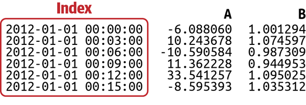
Figure 4-5. The time series index in pandas

This indexing concept can be confusing, so let’s now look at what the alternative is in R and whether that’s better. With the df_ts time series object, there are already a few useful things we can do. It’s also a good starting point when you are working with more advanced time series packages in R because the coercion of a ts object into xts or zoo should throw no errors (this once again is an example of the good object design we covered in Figure 4-3). The first thing you can try to do is plot the object, which often yields good results in R:

plot(df_ts)

Note

Calling the plot function does not simply use a standard function that can plot all kinds of different objects in R (this is what you would expect). It calls a particular method that is associated with the data object (more on the difference between functions and methods is available in Chapter 2). A lot of complexity is hidden behind this simple function call!

The results from plot(df_ts) in Figure 4-6 are already useful. The dates on the x-axis are recognized, and a line plot is chosen instead of the default points plot.

Figure 4-6. Plot of a time-series (ts) object in base R

The most prevalent issue in analyzing time-series data (and most ML data, for that matter) is dealing with noise. The difference between this data format and others is that there are a few different noise sources, and different patterns can be cleaned. This is achieved by a technique called decomposition, for which we have the built-in and well-named function decompose:

decomposed_ts <- decompose(df_ts)
plot(decomposed_ts)

The results can be seen in Figure 4-7.

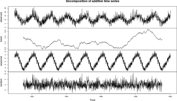
Figure 4-7. Plot of decomposed time-series in base R

We can see what the random noise is and also what is a seasonal and overall pattern. We achieved all this with just one function call in base R! In Python, we would need to use the statsmodels package to achieve the same.

Prophet

For analyzing time-series data, we also have another exciting package example. It’s simultaneously developed for both R and Python (similar to the lime explainable ML tool): Facebook Prophet. This example can help us compare the differences in API design. Prophet is a package whose main strength lies in the flexibility for a domain user to adjust to their particular need, ease of use of the API, and focus on production readiness. These factors make it a good choice for prototyping time series work and using it in a data product. Let’s have a look; our data is stored as a pd.DataFrame in df:

from fbprophet import Prophet

m = Prophet()
m.fit(df) 

future = m.make_future_dataframe(periods=365) 
future.tail()

Here we see the same fit API pattern again, borrowed from scikit-learn.

This step creates a new empty pd.DataFrame that stores our predictions later.

library(prophet)

m <- prophet(df)

future <- make_future_dataframe(m, periods = 365)
tail(future)

Both are simple enough and contain the same number of steps—this is an excellent example of a consistent API design (more on this in Chapter 5).

Tip

It’s an interesting and helpful idea to offer a consistent user experience across languages, but we do not predict it’ll be widely implemented. Few organizations possess the resources to do such work, which can be limiting since compromises have to be made in software design choices.

At this point, you can appreciate that knowing both languages would give you a significant advantage in daily work. If you were exposed only to the Python package ecosystem, you would probably try to find similar tools for analyzing time series and miss out on the incredible opportunities that base R and related R packages provide.

Spatial Data

The analysis of spatial data is one of the most promising areas in modern machine learning and has a rich history. New tools have been developed in recent years, but R has had the upper hand for a long time, despite some recent Python advances. As in the previous sections, we’ll look at a practical example to see the packages in action.

Note

There are several formats of spatial data available. In this subsection, we are focusing on the analysis of raster data. For other formats there are some interesting tools available in Python, such as GeoPandas, but this is out of scope for this chapter.

Our task is to process occurrence (location-tagged observations of the animal in the wild) and environmental data for Loxodonta africana (African elephant) to make it suitable for spatial predictions. Such data processing is typical in species distribution modeling (SDM), where the predictions are used to construct habitat suitability maps used for conservation. This case study is more advanced than the previous ones, and a lot of the steps hide some complexity where the packages are doing the heavy lifting. The steps are as follows:

1. Obtain environmental raster data.

2. Cut the raster to fit the area of interest.

3. Deal with spatial autocorrelation with sampling methods.

To solve this problem as a first step, we need to process raster data.²² This is, in a way, very similar to standard image data, but still different in processing steps. For this R has the excellent raster package available (the alternative is Python’s gdal and R’s rgdal, which in our opinion, are trickier to use).

library(raster)
climate_variables <- getData(name = "worldclim", var = "bio", res = 10)

raster allows us to download most of the common useful spatial environmental datasets, including the bioclimactic data:²³

e <- extent(xmin, xmax, ymin, ymax)
coords_absence <- dismo::randomPoints(climate_variables, 10000, ext = e)
points_absence <- sp::SpatialPoints(coords_absence,
                                    proj4string = climate_variables@crs)
env_absence <- raster::extract(climate_variables, points_absence)

Here we use the handy extent function to crop (cut) the raster data—we are only interested in a subsection of all those environmental layers surrounding the occurrence data. Here we use the longitude and latitude coordinates to draw this rectangle. As a next step, to have a classification problem, we are randomly sampling data points from the raster data (those are called pseudo absences). You could imagine that those are the 0s in our classification task, and the occurrences (observations) are the 1s—the target variable. We then convert the pseudo-absences to SpatialPoints, and finally extract the climate data for them as well. In the SpatialPoints function, you can also see how we specify the geographic projection system, one of the fundamental concepts when analyzing spatial data.

One of the most common issues when working in ML is correlations within the data. The fundamental assumption for a correct dataset is that the individual observations in the data are independent of each other to get accurate statistical results. This issue is always present in spatial data due to its very nature. This issue is called spatial autocorrelation. There are several packages available for sampling from the data to mitigate this risk. One such package is ENMeval:

library(ENMeval)
check1 <- get.checkerboard1(occs, envs, bg, aggregation.factor=5)

The get.checkerboard1 function samples the data in an evenly distributed manner, similar to taking equal points from each square from a black-and-white chessboard. We can then take this resampled data and successfully train an ML model without worrying about spatial autocorrelation. As a final step, we can take those predictions and create the habitat suitability map, shown in Figure 4-8.

raster_prediction <- predict(predictors, model)
plot(raster_prediction)

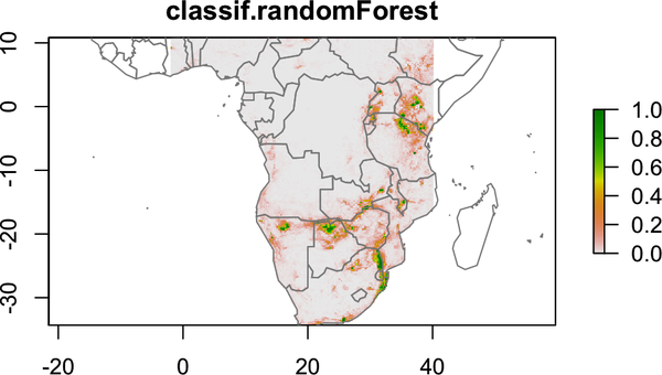
Figure 4-8. Plot of a raster object prediction in R, resulting in a habitat suitability map

When you’re working with spatial raster data, the better package design is provided by R. The fundamental tools such as raster provide a consistent foundation for more advanced application-specific ones such as ENMeval and dismo, without the need to worry about complex transformation or error-prone type coercion.

Final Thoughts

In this chapter we went through the different common data formats and the best packages to process them so they are ready for advanced tasks. In each case study, we demonstrated a good package design and how that can make a data scientist more productive. We have seen that for more ML-focused tasks, such as CV and NLP, Python is providing the better user experience and lower learning curve. In contrast, for more time series prediction and spatial analysis, R has the upper hand. Those selection choices are shown in Figure 4-9.

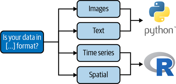
Figure 4-9. Decision tree for package selection

What the best tools have in common is the better package design (Figure 4-3). You should always use the optimal tool for the job and pay attention to the complexity, documentation, and performance of the tools you use!

¹ For a more thorough explanation on this, have a look at RealPython.com’s guide.

² This is commonly referred to as data lineage.

³ Who else didn’t learn what if __name__ == "__main__" does in Python?

⁴ One table from the data, stored in a single file.

⁵ Not to forget readr, which was discussed in Chapter 2.

⁶ We did mention that statisticians are very literal, right?

⁷ This consistency is a common thread in the chapters in Part III and is addressed additionally in Chapter 5.

⁸ Remember—garbage in, garbage out.

⁹ Using code to go through the content of a web page, download and store it in a machine-readable format.

¹⁰ Obtaining more data can be expensive, or even impossible in some cases.

¹¹ If you want to learn more on data augmentation of images, have a look at this tutorial.

¹² At the time of writing.

¹³ Not to be confused with the conference of the same name, the PyData stack refers to NumPy, SciPy, pandas, IPython, and matplotlib.

¹⁴ The R community has also rallied to the call and improved the tooling in recent times, but it still arguably lags behind its Python counterparts.

¹⁵ To learn more about NLTK, have a look at Natural Language Processing with Python by Steven Bird, Ewan Klein, and Edward Loper (O’Reilly), one of the most accessible books on working with text data.

¹⁶ Data type coercion is the conversion of one data type to another.

¹⁷ This is a common step in NLP. Some examples of stop words are “the,” “a,” and “this.” These need to be removed since they rarely offer useful information for ML algorithms.

¹⁸ The process of labeling words with the PoS they belong to.

¹⁹ Converting text into numbers for ingestion by an ML algorithm.

²⁰ Such as trying to create custom embeddings. Check the RStudio blog for more information.

²¹ You can read more about that on the RStudio blog.

²² Data representing cells, where the cell value represents some information.

²³ Environmental features that have been determined by ecologists to be highly predictive of species distributions, i.e., humidity and temperature.