Chapter 4. The Dangers of Conventional Statistical Methodologies

Worse than useless.

—Jerzy Neyman, eminent mathematical statistician, referring to the statistical inference methodology of R. A. Fisher, the chief architect of conventional statistics

Recall from Chapter 1 that all financial models are at the mercy of the trifecta of errors, namely: errors in model specifications; errors in model parameter estimates; and errors resulting from the failure of a model to adapt to structural changes in its environment. Because of these errors, we need dynamic models that quantify the uncertainty inherent in our financial inferences and predictions.

A statistical inference methodology known as null hypothesis significance testing (NHST) almost completely dominates the research and practice of social and economic sciences. In this chapter, we examine how NHST and its p-value statistic is used for testing hypotheses and quantifying uncertainty of model parameters. The deep logical flaws of NHST methodology are primarily responsible for the reproducibility crisis in all the social and economic sciences, where the majority of published research findings are false.¹ In the next couple of sections, we expose the statistical skullduggery of NHST and its p-value statistic and show you how it is guilty of the prosecutor’s fallacy. This fallacy is another version of the inverse fallacy, where a conditional statement is falsely equated with its inverse, thereby violating the inverse probability rule.

Given the deep flaws and abuses of p-values for quantifying parameter uncertainty,² another methodology known as confidence intervals (CIs) is touted by orthodox statisticians as its mathematically rigorous replacement. Unfortunately, CIs are also the wrong tool for data analysis, since they were not designed to make statistical inferences from a single experiment.³ Most importantly, the application of CIs in finance often violates the assumptions of the central limit theorem (CLT), making CIs invalid. In this chapter, we explore the trio of errors in applying CIs that are common in financial research and practice. We develop an ordinary least squares (OLS) linear regression model of equity returns using Statsmodels, a Python statistical package, to illustrate these three error types. We use the diagnostic test results of our regression model to support our reasons why CIs should not be used in data analyses in general and finance in particular.

The Inverse Fallacy

Recall the proof of the inverse probability rule, a trivial reformulation of the product rule. For any nonzero probability event H and D:

P(H and D) = P(D and H) (product of probabilities commute)
P(H|D) × P(D) = P(D|H) × P(H) (applying product rule to both sides)
P(H|D) = P(D|H) × P(H) / P(D) (the inverse probability rule)

Note that joint probabilities, the product of two probabilities, commute—i.e., the order of the individual probabilities does not change the result of their product:

P(H and D) = P(D and H)

As you can see from the last equation, conditional probabilities do not commute:

P(H|D) ≠ P(D|H)

This is a common logical mistake that people make in their thinking and scientists continue to make in their research when using NHST and p-values. This is called the inverse fallacy because you are incorrectly equating a conditional probability, P(D|H), with its inverse, P(H|D), and violating the inverse probability rule. The inverse fallacy is also known as transposed conditional fallacy. As a simple example, consider how the inverse fallacy incorrectly infers statement B from statement A:

(A) Given that someone is a programmer, it is likely that they are analytical.
(B) Given that someone is analytical, it is likely that they are a programmer.

But P(analytical | programmer) ≠ P(programmer | analytical). As you know, there are many, many analytical people who are not programmers, and such an inference seems absurd when framed in this manner. However, you will see that humans are generally not very good at processing conditional statements and their inverses, especially in complex situations. Indeed, prosecutors have ruined people’s lives by using this flawed logic disguised in arguments that have led judges and juries to make terrible inferences and decisions.⁴ A common example of the prosecutor’s fallacy goes something like this:

(A) Say about 0.1% of the 100,000 adults in your city have your blood type.
(B) A blood stain with your blood type is found on the murder victim.
(C) Therefore, claims the city prosecutor, there is a 99.9% probability that you are the murderer.

That’s clearly absurd. What is truly horrifying—and we should all be screaming bloody murder—is that researchers and practitioners are unknowingly using the prosecutor’s fallacious logic when applying NHST and p-values in their statistical inferences. More on NHST in the next section. Let’s expose the prosecutor’s flawed reasoning in this section so that you can see how it is used in the NHST methodology.

The probability of your guilt (G) before the blood stain evidence (E) was discovered to be P(G) = 1/100,000, since every adult in the city is an equally likely suspect. Therefore, the probability of your innocence (I) is P(I) = 99,999/100,000. The probability that the blood stain would match your blood type given you are actually guilty is a certainty, implying P(E | G) = 1. However, even if you are actually innocent, there is still a 0.1% probability that the blood stain would match your blood type merely by its prevalence in the city’s adult population, implying P(E | I) = 0.001. The prosecutor needs to estimate P(G | E), the probability of your guilt given the evidence, with the previously mentioned probabilities. Instead of using the inverse probability rule, the prosecutor uses a fallacious argument as follows:

(A) Given the evidence, you can be either guilty or innocent, so P(G | E) + P (I | E) = 1
(B) Now the prosecutor commits the inverse fallacy by making P(I | E) = P(E | I)
(C) Thus the prosecutor’s fallacy gives you P (G | E) = 1 – P(I | E) = 1 – P(E | I)
(D) Plugging in the numbers, P(G | E) = 1 – 0.001 = 0.999 or 99.9%

Without explicitly using the inverse probability rule, your lawyer could use some common sense and correctly argue that there are 100 adults (0.1% × 100,000) in the city who have the same blood type as you do. Therefore, given evidence of the blood stain alone, there is only a 1 in 100 chance or 1% probability that you are guilty and 99% probability that you are innocent. This is approximately the same probability you would get when applying the inverse probability rule because it just formulates a commonsensical way of counting the possibilities. Let’s do that now and calculate the probability of your innocence given the evidence, P(I | E):

(A) The inverse probability rule states P (I | E) = P(E | I) × P(I)/ P(E)
(B) We use the law of total probability to get P(E) = P(E | I) × P(I) + P(E | G) × P(G)
(C) So P(I | E) = 0.001 × 0.99999 / [(0.001 × 0.99999) + ( 1 × 0.00001)] = 0.99 or 99%

Before the prosecutor strikes you off the suspect list, it is important to note that it would also be fallacious for your lawyer to now ask the jury to disregard the blood stain as weak evidence of your guilt based on the 1% conditional probability just calculated. This flawed line of reasoning is called the defense attorney’s fallacy and was used in the notorious O. J. Simpson murder trial. The evidence is not weak, because before the blood stain was found, you had a 1 in 100,000 chance of being the murderer. But after the blood stain was discovered, your chance of being guilty has gone up a thousand times to 1 in 100. That’s very strong evidence indeed and nobody should disregard it. However, it is completely inadequate for a conviction if that is the only piece of evidence presented to the jury. The prosecutor will need additional incriminating evidence to make a valid case against you.

Now let’s look at a realistic financial situation where the inverse fallacy might be harder to spot. Economic recessions are notoriously hard to recognize in the early stages of their development. As I write this chapter (in the fall of 2022), there is a debate raging among economists and investors about whether the US economy is currently in a recession or about to enter one. Economists at the National Bureau of Economic Research (NBER), the organization responsible for making the recession official, can only confirm the fact in retrospect. Sometimes the NBER takes over a year to declare when the recession actually started, as it did in the Great Recession of 2007–09. Of course, traders and investors cannot wait that long, and they develop their own indicators for predicting recessions in real time.

Assume that you have developed a proprietary economic indicator that crunches all kinds of data and correctly signals a recession 99% of the time when the US economy is actually in one or about to enter one. You also note that about 20% of the time your indicator signals a recession incorrectly even though the economy is not in one. Say you just found out that your proprietary indicator is flashing a recession signal. What is the probability that the US economy has actually entered into a recession? If you answered that the probability is 99%, as many people instinctively do, you would have committed the inverse fallacy since P(recession given signal) ≠ P(signal given recession).

Let’s see why the probability of recession is not 99% but much lower. Assume R is the scenario that the US economy is in a recession and S is the event that your indicator signals that we are in a recession. You have the following conditional probabilities:

The probability of your indicator giving you a recession signal given we actually are in one is P(S|R) = 0.99 or 99%. This is its true positive rate.
This implies that the probability your indicator fails to detect a recession given we are actually in one, P(not S|R) = 1 – P(S|R) = 0.01 or 1%. This is its false negative rate.
The probability your indicator incorrectly alerts you to a recession when there isn’t one is P(S|not R) = 0.20 or 20%. This is its false positive rate.
Similarly, the probability that your indicator successfully detects that the economy is not in a recession, P(not S| not R) = 1 – P(S|not R) = 0.80 or 80%. This is its true negative rate.

These conditional probabilities are generally organized in a confusion matrix, as shown in Figure 4-1.

Your objective is to estimate P(R|S), the conditional probability that the US economy is in a recession, given your indicator generates such a signal. To calculate this inverse probability P(R|S), you can’t only let the data speak about one specific scenario. Why? Because your economic indicator does not have 100% accuracy. It gives you a false recession signal 20% of the time when the economy is not in one. Could this scenario be 1 of the 5 when it is wrong about the economy being in a recession? Also, 1% of time it fails to detect a recession when the economy is actually in one. So maybe we have already been in a recession for many months, and it is 1 of the 100 instances when your indicator failed to flicker. How would you know just from the data about this particular scenario? You wouldn’t, because you don’t have a clue about the environment you are operating in. You need to leverage prior knowledge so that you can understand the context in which you are running your financial experiments.

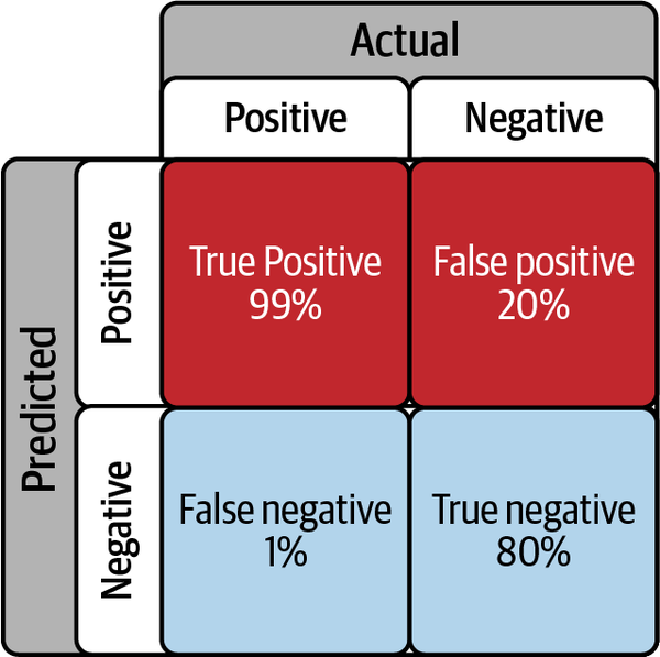
Confusion Matrix of your proprietary recession indicator

Your specific dataset is oblivious of how common or uncommon recessions are in the US. Why is that relevant? Because you don’t know if your false positive rate is too high, or low enough, compared to the rate at which recessions tend to occur in the US for your indicator to be useful, despite its 99% true positive rate.

You will need to estimate the probability that the US could be in a recession in any given month P(R) based on past occurrences; this is called the base rate of the particular event/scenario R. Ignoring the base rate leads to a violation of the inverse probability rule and invalid inferences, as we will demonstrate.

Let’s compute the base rate from actual economic data. The NBER’s time series for every month since 1982 that the US was in an economic recession can be downloaded from Federal Reserve Economic Data (FRED), a popular and free data source that has more than half a million economic and financial time series. Let’s use the following Python code to calculate the monthly base rate of economic recessions in the US:

# Import libraries and FRED datareader
import numpy as np
import pandas as pd
import pandas_datareader.data as pdr
from datetime import datetime
start = datetime(1982, 1, 1)
end = datetime(2022, 9, 30)
# NBER business cycle classification
recession = pdr.DataReader('USREC', 'fred', start, end)
# Percentage of time the US economy was in recession since 1982
round(recession['USREC'].sum()/recession['USREC'].count()*100, 2)

From this data, the US has been in an economic recession only 9.61% of the time in any given month from January 1982 to September 2022. Once you have estimated P(R), you can plug it into the law of total probability to get the unconditional probability, or marginal probability P(S), of getting a recession signal from your indicator regardless of the state of the economy. We then use P(R) in the inverse probability rule to calculate the probability the US economy is in recession, given that your proprietary indicator is signaling a recession:

P(S) = P(S|R) × P(R) + P(S|not R) × P(not R) = (0.99 × 0.096) + (0.2 × 0.904) = 0.276
P(R|S) = P(S|R) × P(R) / P(S) = (0.99 × 0.096) / 0.276 = 0.344

The calculation for P(S) says that you can expect your indicator to generate a signal 27.6% of the time regardless of whether the US economy is in a recession or not. Of the times you do see it flicker, P(R|S) says that in only 34.4% of those scenarios will the signal be correct about the economy being in a recession. Your signal will give you a false alarm P(not R|S) about 65.6% of the time. That’s a very poor indicator—you’re better off ignoring it.

This result seems counterintuitive since your indicator has a 99% true positive rate P(S|R). That’s because you cannot shove your indicator’s false positive rate under the rug and blithely ignore the base rate of US economic recessions with some ideological rubbish of being objective and letting only the data speak. That would be foolish because you would be denying the inverse probability rule and ignoring objective prior data about US economic cycles. Such fallacious inferences and decision making will almost surely see you go broke or be out of a job sooner rather than later.

In the real world of finance and investing, you will need a signal with a false positive rate lower than the base rate to give you a signal with a probability greater than 50% of being correct. To see this, let’s redo the calculation with a revised false positive of 9%, which is slightly less than the 9.61% base rate at which the US economy has been in a recession in any given month since 1982:

P(S) = P(S|R) × P(R) + P(S|not R) × P(not R) = (0.99 × 0.096) + (0.09 × 0.904) = 0.176
P(R|S) = P(S|R) × P(R) / P(S) = (0.95 × 0.0967)/0.174 = 0.540

With a 54% probability of correctly calling a recession, your indicator will have an edge or positive expectation for better decision making and risk management.

To summarize, the true positive rate of your indicator is important. However, what is equally important is that the false positive rate of the indicator needs to be less than the base rate of the underlying feature in the population you are sampling from. So if you ignore the fact that your indicator is generating false positives P(S|not R) at a 20% rate while the US economy is generating a recessionary month at a 9.61% base rate, your false positives will overwhelm your true positives at a 2 to 1 ratio. It doesn’t seem so far-fetched now to think that unscrupulous prosecutors, snake oil salesmen, and pseudoscientists could fool you (and themselves) with the inverse fallacy.

Since there is still a 34.4% chance that your indicator might be right, randomness could also fool you, too, by granting you a lucky guess, and the US economy could end up being in a recession. However, your probability estimate of 99% would be way off, and your reasoning would be fallacious. A trading or investing strategy based on luck, incorrect reasoning, and poor probability estimates will lead to financial ruin sooner rather than later. Far worse, a statistical methodology like NHST based on the inverse fallacy will overwhelm us with false positive studies, creating confusion and harm. This will ruin the scientific enterprise that we cherish and value so much.

NHST Is Guilty of the Prosecutor’s Fallacy

Ronald Fisher, the head architect of modern statistics, introduced NHST in the 1920s. He also included Karl Pearson’s p-value into his methodology for quantifying uncertainty. This was a postdata methodology and was meant to enable researchers to make statistical inferences from a single experiment based on a null hypothesis that is the negation of the hypothesis that the researcher is trying to prove.

In 1925, Fisher made the absurd and unsubstantiated claim that “the theory of inverse probability is founded upon error and must be wholly rejected.”⁶ Of course Fisher didn’t and couldn’t provide any proof for this claim. How could he? That would be akin to proving the rules of division are founded on error. As mentioned in the previous chapter, my suspicion is that by renaming the rule after an amateur mathematician, Thomas Bayes, he could cast aspersions on the rule. By rejecting the inverse probability rule, Fisher was able to use the prosecutor’s fallacy to promote his flawed discriminatory ideas under the guise of objectivity and “letting the data speak for themselves.”⁷ Fisher’s fawning cohorts in industry and slavish acolytes in academia merely repeated the lie about the inverse probability theory and banished it from their practice and curricula—a problem that continues to this day.

NHST is built behind the facade of a valid form of propositional logic known as proof by contrapositive. The logic is as follows: suppose we have two propositions H and D such that if H is true, then D is true. Now if we can prove that D is false, then we can validly conclude that H must be false.

Following the latter logic, researchers using NHST formulate a hypothesis, called the null hypothesis (H₀), that they want to disprove before observing any data. H₀ is viewed as the negation of an alternative research hypothesis (H₁) that they want to establish but is not explicitly specified, i.e., H₁ = not H₀ and P(H₁) + P(not H₀) = 1. In this regard, they play the devil’s advocate for the null hypothesis.

The null hypothesis is generally formulated as a summary statistic, such as the difference in the sample means of the data distribution of two groups that need to be compared. It is important to note that researchers do not predict the data that their research hypothesis H₁ is expected to generate, assuming that H₁ is true.

Before starting their experiment, researchers also choose a significance level, denoted by alpha, which works as a decision threshold to accept or reject the null hypothesis after observing the data. The convention is to set alpha to 5%. The alpha level is claimed to be the long-run probability that the researcher might incorrectly reject a true null hypothesis, thereby committing a type I error and generating false positive results (a result that is claimed to be true when it is actually false). The alpha level is the most critical element of the experiment, since it determines if the experiment is considered statistically significant or not.

It is important to note that any significance level is entirely subjective, as it is not based on the observed data or the null hypothesis or a scientific reason or any mathematical rule or theorem. The conventional use of the 5% alpha level is a totally arbitrary and self-fulling ritual. Since Fisher used a 5% alpha significance level, researchers and academics blindly follow his example. So much for the vaunted objectivity and scientific rigor of frequentists, not to mention letting the data speak for themselves.

Assuming the null hypothesis is true, the researcher computes a statistic called the p-value to quantify the probability of observing the summary statistic of the sample data (D) or something more extreme than it:

p-value = P(D|H₀)

If the p-value ≤ alpha, H₀ is rejected as false at the alpha significance level and the alternative hypothesis (H₁) is accepted as true.

But this logic of NHST is mind-bogglingly absurd. By rejecting the null hypothesis (H₀) given the p-value of the test statistic (D), the researcher is committing the inverse fallacy, because P(H₀ | D) ≠ P(D | H₀). See Figure 4-2.

NHST makes an even more absurd leap of logic. NHST commits the prosecutor’s fallacy by allowing researchers to accept the unspecified, alternative research hypothesis, which the data was not modeling in the first place. Go back to the previous section and refresh your memory about how we disentangled the prosecutor’s fallacy.

The researcher wants to determine P(H₁|D), the probability the research hypothesis (H₁) is true given the data. But NHST only computes P(D|H₀), the probability of observing the data assuming the null hypothesis (H₀) is true. It then uses the p-value statistic to accept or reject the null hypothesis at the alpha significance level. So researchers following the NHST methodology commit the prosecutor’s fallacy as follows:

P(H₁|D) = 1 – P(H₀|D) (true statement)
P(H₀|D) = P(D|H₀) (the inverse fallacy)
P(H₁|D) = 1 – P(D|H₀) (the prosecutor’s fallacy)

How should we validly calculate P(H₁|D)? The binary logic of proof by contrapositive in a deterministic world needs to be translated into the calculus of conditional probabilities in an uncertain world. This translation is enabled by the inverse probability rule and the law of total probability, as was applied in the previous section:

P(H₁|D) = 1 – P(H₀|D)
P(H₁|D) = 1 – [P(D|H₀)P(H₀)/P(D)]
P(H₁|D) = 1 – [P(D|H₀)P(H₀) / (P(D|H₀)P(H₀) + P(D|H₁)P(H₁))]

As this equation, which I have derived, shows, the researcher needs to estimate P(D|H₁), the probability of observing the data assuming their research hypothesis H₁ is true. Most importantly, the researcher needs to estimate the prior probability or base rate of at least one of their complementary hypotheses, P(H₀) or P(H₁). That’s because without the base rate, you cannot compute the evidence or the unconditional probability of observing the data. This fallacious logic is what makes statistical inferences about either the null hypothesis or the alternative research hypothesis invalid. It is for very good reasons that Jerzy Neyman, an eminent statistician and Fisher’s peer, called Fisher’s work on statistical inference “worse than useless.”⁹

It is clear that NHST—the cornerstone of education, research, and practice of the social and economic sciences—is committing the prosecutor’s fallacy. No wonder most of the published research findings using NHST are false. NHST has wasted billions of research dollars, defamed science, and done a great disservice to humanity with its false positive research studies. All this while professing the farce of rigor and objectivity. NHST continues to wreak havoc on the social and economic sciences, producing too many false research claims to this day despite many failed attempts to abolish it or reform it for over half a century.¹⁰ It’s about time we reject the NHST because it “is founded upon error and must be wholly rejected.”¹¹

Many in the social and economic sciences recommend replacing p-values with CI theory, which is touted as a mathematically more rigorous way of quantifying uncertainty. So let’s examine CI theory to see if it is useful.

How Null Hypothesis Significance Testing Became “Worse Than Useless”

Soon after Fisher introduced NHST, Jerzy Neyman and Egon Pearson, the other two architects of modern statistics, introduced their methodology of statistical hypothesis testing as a decision framework for industrial quality control.

There was a bitter rivalry between Fisher and Neyman as they advocated for their respective methodologies. Neyman called Fisher’s statistical work “worse than useless,” and Fisher called Neyman’s work “childish” and “horrifying.” Unfortunately, both Neyman and Fisher were right. Fisher’s work on statistical inference is indeed worse than useless because he rejected the inverse probability rule and unabashedly committed the prosecutor’s fallacy with impunity.

Fisher was right in that Neyman’s work is not applicable to social sciences but to industrial quality control. It would be inappropriate to apply it to social systems of creative and free-willed humans instead of factory widgets. Fisher also didn’t understand that Neyman’s theory was a predata theory, and it would be absurd if it were applied as a postdata theory of statistical Inference.

As the two competing methodologies spread throughout the social and economic sciences in the last century, researchers tried to reconcile the ideas of the two bitter rivals. Unfortunately, these social scientists and statisticians did not have a deep understanding of either methodology.¹² This inept fusion of the two methodologies is how NHST became “worse than useless.”

The Confidence Game

As mentioned in the previous sidebar, Jerzy Neyman developed a statistical decision theory designed to support industrial quality control. His statistical theory provides a decision framework that seeks to control type I (false positive) and type II (false negative) errors to balance costs versus benefits over the long run based on many experiments. Neyman intentionally left out p-values because it was a nonsensical concept violating basic probabilistic logic.

In 1937, Neyman developed CI theory to be a predata theory of statistical inference, intended to inform statistical procedures that have long-run average properties before data are sampled from a population distribution. Neyman made it very clear that his CI theory was not intended to support inferences after data are sampled in a single scientific experiment. CI theory is not a postdata theory of statistical inference despite how it is applied today in research and practice in social and economic sciences.

CI theory quantifies uncertainty of population parameter estimates. For example, a 90% confidence interval (CI), as shown in Figure 4-3, is generally understood to imply that there is a 90% probability that the true value of a parameter of interest is in the interval [–a, a].

The interval [–a, a] is called a 90% confidence interval.

Fisher attacked Neyman’s CI theory by claiming it did not serve the needs of scientists and potentially would lead to mutually contradictory inferences from data. Fisher’s criticisms of CI theory have proven to be justified—but not because Neyman’s CI theory is logically or mathematically flawed, as Fisher claimed.

Let’s examine the trio of errors that arise from the common practice of misusing Neyman’s CI theory as a postdata theory—i.e., for making inferences about population parameters based on a specific data sample. The three types of errors using CIs are:

Making probabilistic claims about population parameters
Making probabilistic claims about a specific confidence interval
Making probabilistic claims about sampling distributions

The frequentist philosophy of probability and statistical inference has had a profound impact on the theory and practice of financial economics in general and CIs in particular. To explore the implications of confidence intervals (CIs) for our purposes, we begin the next subsection by discussing the fundamental concepts of a simple market model and its relationship to financial theory. Afterward, we utilize Statsmodels, a statistical package in Python, to construct an ordinary least squares (OLS) linear regression model of equity returns to estimate the parameters of our market model. This real-world example allows us to illustrate how CIs are actually applied in financial data analysis. In the next sections, we examine why CIs are logically incoherent and practically useless.

Single-Factor Market Model for Equities

Modern portfolio theory assumes that rational, risk-averse investors demand a risk premium, a return in excess of a risk-free asset such as a treasury bill, for investing in risky assets such as equities. A stock’s single-factor market model (MM) is basically a linear regression model of the realized excess returns of a stock (outcome or dependent variable) regressed against the realized excess returns of a single risk factor (predictor or independent variable) such as the overall market, as formulated here:

( R − F ) = α + β × ( M − F ) + ϵ

Where R is the realized return of a stock, F is the return on a risk-free asset such as a US Treasury security, M is the realized return of a market portfolio such as the S&P 500, α (alpha) is the expected stock-specific return, β (beta) is the level of systematic risk exposure to the market, and ε (epsilon) is the unexpected stock-specific return. The beta of a stock gives the average percentage return response to a 1% change in return of the overall market portfolio. For example, if a stock has a beta of 1.4 and the S&P 500 falls by 1%, the stock is expected to fall by –1.4% on average. See Figure 4-4.

Market Model showing the excess returns of Apple Inc. (AAPL) regressed against the excess returns of the S&P 500

Note that the MM of an asset is different from its capital asset pricing model (CAPM). The CAPM is the pivotal economic equilibrium model of modern finance that predicts expected returns of an asset based on its β or systematic risk exposure to the overall market. Unlike the CAPM, an asset’s MM is a statistical model about realized returns that has both an idiosyncratic risk term ɑ and an error term ɛ in its formulation.

According to the CAPM, the alpha of an asset’s MM has an expected value of zero because market participants are assumed to hold efficient portfolios that diversify the idiosyncratic risks of any specific asset. Market participants are only rewarded for bearing systematic risk since it cannot be diversified away. In keeping with the general assumptions of an OLS regression model, both CAPM and MM assume that the expected value of the residuals ɛ will be normally distributed with a zero mean and a constant, finite variance.

A financial analyst, relying on modern portfolio theory and practice, assumes there is an underlying, time-invariant, stochastic process generating the price data of Apple Inc., which can be modeled as an OLS linear regression MM. This MM will have population parameters, alpha and beta, which have true, fixed values that can be estimated from reason random samples of Apple’s closing price data.

Simple Linear Regression with Statsmodels

Let’s run our Python code to estimate alpha and beta based on a sample of five years of daily closing prices of Apple. We can use any holding period return as long as it is used consistently throughout the formula. Using a daily holding period is convenient because it makes price return calculations much easier using pandas DataFrames:

# Install Yahoo finance package
!pip install yfinance

# Import relevant Python packages
import statsmodels.api as sm
import pandas as pd
import yfinance as yf

import matplotlib.pyplot as plt
plt.style.use('seaborn')
from datetime import datetime
#Import financial data
start = datetime(2017, 8, 3)
end = datetime(2022, 8, 6)

# S&P 500 index is a proxy for the market
market = yf.Ticker('SPY').history(start=start, end=end)
# Ticker symbol for Apple, the most liquid stock in the world
stock = yf.Ticker('AAPL').history(start=start, end=end)
# 10 year US treasury note is the proxy for risk free rate
riskfree_rate = yf.Ticker('^TNX').history(start=start, end=end)
# Create dataframe to hold daily returns of securities
daily_returns = pd.DataFrame()
daily_returns['market'] = market['Close'].pct_change(1)*100
daily_returns['stock'] = stock['Close'].pct_change(1)*100
# Compounded daily rate based on 360 days 
# for the calendar year used in the bond market
daily_returns['riskfree'] = (1 + riskfree_rate['Close']) ** (1/360) - 1
# Plot and summarize the distribution of daily returns
plt.hist(daily_returns['market']), plt.title('Distribution of Market (SPY) 
Daily Returns'), plt.xlabel('Daily Percentage Returns'), 
plt.ylabel('Frequency'), plt.show()
# Analyze descriptive statistics
print("Descriptive Statistics of the Market's daily percentage returns:\n{}".
format(daily_returns['market'].describe()))

plt.hist(daily_returns['stock']), 
plt.title('Distribution of Apple Inc. (AAPL) Daily Returns'), 
plt.xlabel('Daily Percentage Returns'), plt.ylabel('Frequency'), plt.show()
# Analyze descriptive statistics
print("Descriptive Statistics of the Apple's daily percentage returns:\n{}"
.format(daily_returns['stock'].describe()))

plt.hist(daily_returns['riskfree']), plt.title('Distribution of the riskfree 
rate (TNX) Daily Returns'), plt.xlabel('Daily Percentage Returns'), 
plt.ylabel('Frequency'), plt.show()
# Analyze descriptive statistics
print("Descriptive Statistics of the 10 year note daily percentage returns:\n{}"
.format(daily_returns['riskfree'].describe()))
# Examine missing rows in the dataframe
market.index.difference(riskfree_rate.index)
# Fill rows with previous day's risk-free rate since daily rates 
# are generally stable
daily_returns = daily_returns.ffill()
# Drop NaNs in first row because of percentage calculations
daily_returns = daily_returns.dropna()
# Check dataframe for null values
daily_returns.isnull().sum()
# Check first five rows of dataframe
daily_returns.head()
# AAPL's Market Model based on daily excess returns

# Daily excess returns of AAPL
y = daily_returns['stock'] - daily_returns['riskfree']
# Daily excess returns of the market
x = daily_returns['market'] - daily_returns['riskfree']

# Plot the data
plt.scatter(x,y)

# Add the constant vector to obtain the intecept
x = sm.add_constant(x)

# Use ordinary least squares algorithm to find the line of best fit
market_model = sm.OLS(y, x).fit()

# Plot the line of best fit
plt.plot(x, x*market_model.params[0]+market_model.params['const'])
plt.title('Market Model of AAPL'), plt.xlabel('SPY Daily Excess Returns'), 
plt.ylabel('AAPL Daily Excess Returns'), plt.show();

# Display the values of alpha and beta of AAPL's market model
print("According to AAPL's Market Model, the security had a realized Alpha of 
{0}% and Beta of {1}".format(round(market_model.params['const'],2), 
round(market_model.params[0],2)))
# Summarize and analyze the statistics of your linear regression
print("The Market Model of AAPL is summarized below:\n{}"
.format(market_model.summary()));

After running our Python code, a financial analyst would estimate that alpha is 0.071% and beta is 1.2385, as shown in the Statsmodels summary output:

The Market Model of AAPL is summarized below:
OLS Regression Results
=========================================================================
Dep. Variable:      y                       R-squared:          0.624
Model:              OLS                     Adj. R-squared:     0.624
Method:             Least Squares           F-statistic:        2087.
Date:               Sun, 07 Aug 2022        Prob (F-statistic): 2.02e-269
Time:               06:28:33                Log-Likelihood:     -2059.8
No. Observations:   1260                    AIC:                4124.
Df Residuals:       1258                    BIC:                4134.
Df Model:           1
Covariance Type:    nonrobust 
========================================================================
        coef        std err     t        P>|t|     [0.025      0.975]
const   0.0710      0.035     2.028      0.043     0.002       0.140
0       1.2385      0.027     45.684     0.000     1.185       1.292
========================================================================
Omnibus:        202.982             Durbin-Watson:          1.848
Prob(Omnibus):  0.000               Jarque-Bera (JB):       1785.931
Skew:           0.459               Prob(JB):               0.00
Kurtosis:       8.760               Cond. No.               1.30
======================================================================
Warnings:
[1] Standard Errors assume that the covariance matrix of the errors 
is correctly specified.

Confidence Intervals for Alpha and Beta

Clearly, these point estimates of alpha and beta will vary depending on the sample size as well as start and end dates used in our random samples, with each estimate reflecting Apple’s idiosyncratic price fluctuations during that specific time period. Even though the population parameters alpha and beta are unknown, and possibly unknowable, the financial analyst considers them to be true constants of a stochastic process. It is the random sampling of Apple’s price data that introduces uncertainty in the estimates of constant population parameters. It is the data, and every statistic derived from the data, such as CIs, that are treated as random by frequentists. Financial analysts calculate CIs from random samples to express the uncertainty around point estimates of constant population parameters.

CIs provide a range of values with a probability value or significance level attached to that range. For instance, in Apple’s MM, a financial analyst could calculate the 95% confidence interval by calculating the standard error (SE) of alpha and beta. Since the residuals ɛ are assumed to be normally distributed with an unknown, constant variance, the t-statistic would need to be used in computing CIs. However, because the sample size is greater than 30, the t-distribution converges to the standard normal distribution, and the t-statistic values are the same as the Z-scores of a standard normal distribution. So the analyst would multiply each SE by +/– the Z-score for a 95% CI and then add the result to the point estimate of alpha and beta to obtain its CI. From the previous Statsmodels regression results, the 95% CI for alpha and beta were computed as follows:

α+/– (SE × t-statistic / Z-score for 95% CI) = 0.0710 % +/– (0.035 % × 1.96) = [0.002%, 0.140%]
β+/- (SE × t-statistic / Z-score for 95% CI) = 1.2385 +/– (0.027 × 1.96) = [1.185, 1.292])

Unveiling the Confidence Game

To understand this trio of errors, we need to understand probability and statistical inference from the perspective of a modern statistician. As discussed in Chapter 2, frequentists, such as Fisher and Neyman, claim that probability is a natural, static property of an event and is measured empirically as its long-run relative frequency.

Frequentists postulate that the underlying stochastic process that generates data has statistical properties that do not change in the long run: the probability distribution is stationary ergodic. Even though the parameters of this underlying process may be unknown or unknowable, frequentists believe that these parameters are constant and have “true” values. Population parameters may be estimated from random samples of data. It is the randomness of data that creates uncertainty in the estimates of the true, fixed population parameters.

What most people think they are getting from a 95% CI is a 95% probability that the true population parameter is within the limits of the specific interval calculated from a specific data sample. For instance, based on the Statsmodels results, you would think there is a 95% probability that the true value of beta of Apple is in the range [1.185, 1.292]. Strictly speaking, your interpretation of such a CI would be wrong.

According to Neyman’s CI theory, what a 95% CI actually means is that if we were to draw 100 random samples from Apple’s underlying stock return distribution, we would end up with 100 different confidence intervals, and we can be confident that 95 of them will contain the true population parameter within their limits. However, we won’t know which specific 95 CIs of the 100 CIs include the true value of the population parameter and which 5 CIs do not. We are assured that only the long-run ratio of the CIs that include the population parameter to the ones that do not will approach 95% as we draw random samples ad nauseam.

Winston Churchill could just as well have been talking about CIs instead of Russia’s world war strategy when he said, “It is a riddle, wrapped in a mystery, inside an enigma; but perhaps there is a key.” Indeed, we do present a key in this chapter. Let’s investigate the triumvirate of fallacies that arise from misusing CI as a postdata theory in financial data analysis.

Errors in Making Probabilistic Claims About Population Parameters

Recall that a frequentist statistician considers a population parameter to be a constant with a “true” value. This value may be unknown or even unknowable. But that does not change the fact that its value is fixed. Therefore, a population parameter is either in a CI or it is not. For instance, if you believe the theory that capital markets are highly efficient, you would also believe that the true value of alpha is 0. Now 0 is definitely not in the interval [0.002%, 0.14%] calculated in the previous Statsmodels regression results. Therefore, the probability that alpha is in our CI is 0% and not 95% or any other value.

Because population parameters are believed to be constants by frequentists, there can be absolutely no ambiguity about them: the probability that the true value of a population parameter is within any CI is either 0% or 100%. So it is erroneous to make probabilistic claims about any population parameter under a frequentist interpretation of probability.

Errors in Making Probabilistic Claims About a Specific Confidence Interval

A more sophisticated interpretation of CIs found in the literature and textbooks goes as follows: hypothetically speaking, if we were to repeat our linear regression many times, the interval [1.185, 1.292] would contain the true value of beta within its limits about 95% of the time.

Recall that probabilities in the frequentist world apply only to long-run frequencies of repeatable events. By definition, the probability of a unique event, such as a specific CI, is undefined and makes no sense to a frequentist. Therefore, a frequentist cannot assign a 95% probability to either of the specific intervals for alpha and beta that we have calculated. In other words, we can’t really infer much from a specific CI.

But that is the main objective of our exercise! This limitation of CIs makes it utterly useless for data scientists who want to make inferences about population parameters from their specific data samples: i.e., they want to make postdata inferences. But, as was mentioned earlier, Neyman intended his CI theory to be used for only predata inferences based on long-term frequencies.

Errors in Making Probabilistic Claims About Sampling Distributions

How do financial analysts justify making these probabilistic claims about CIs in research and practice? How do they square the circle? What is the key to applying CIs in a commonsensical way? Statisticians can, in theory or in practice, repeatedly sample data from a population distribution. The point estimates of sample means computed from many different random samples create a pattern called the sampling distribution of the sample mean. Sampling distributions enable frequentists to invoke the central limit theorem (CLT) in calculating the uncertainty around sample point estimates of population parameters. In particular, as was discussed in the previous chapter, the CLT states that if many samples are drawn randomly from a population with a finite mean and variance, the sampling distribution of the sample mean approaches a normal distribution asymptotically. The shape of the underlying population distribution is immaterial and can only affect the speed of this inexorable convergence to normality. See Figure 3-7 in the previous chapter.

The frequentist definition of probability as a long-run relative frequency of repeatable events resonates with the CLT’s repeated drawing of random samples from a population distribution to generate its sampling distributions. So statisticians square the circle by invoking the CLT and claiming that their sampling distributions almost surely converge to a normal distribution, regardless of the shape of the underlying population distribution. This also enables them to compute CIs using the Z-scores of the standard normal distribution, as shown in the previous Statsmodels regression results. This is the key to the enigmatic use of CI as a postdata theory.

However, as financial executives and investors putting our capital at risk, we need to read the fine print of the CLT: specifically, we need to note its assumption that the underlying population distribution needs to have a finite mean and variance. While most distributions satisfy these two conditions, there are many that do not, especially in finance and economics. For these types of population distributions, the CLT cannot be invoked to save CIs. The key does not work on these doors—it is not a magic key. For instance, the Cauchy and Pareto distributions are fat-tailed distributions that do not have finite means or variances. As was mentioned in the previous chapter and is worth repeating, a Cauchy (or Lorentzian) distribution looks deceptively similar to a normal distribution, but has very fat tails because of its infinite variance. See Figure 4-5.

The diagnostic tests computed by Statsmodels in Figure 4-4 show us that the equity market has wrecked the key assumptions of our MM. Specifically, the Bera-Jarque and Omnibus normality tests show the probability that the residuals ɛ that are normally distributed are almost surely zero. This distribution is positively skewed and has very fat tails—a kurtosis that is about three times that of a standard normal distribution.

Compare Cauchy/Lorentzian distribution with the Normal distribution.

How about making the sample size even larger? Won’t the distribution of the residuals get more normal with a much larger sample size, as claimed by financial theory? Let’s run our MM using 25 years of Apple’s daily closing prices—a quarter of a century’s worth of data. Here are the results:

The Market Model of AAPL is summarized below:
OLS Regression Results
=========================================================================
Dep. Variable:      y                       R-squared:          0.270
Model:              OLS                     Adj. R-squared:     0.270
Method:             Least Squares           F-statistic:        2331.
Date:               Sun, 07 Aug 2022        Prob (F-statistic): 0.00
Time:               07:03:34                Log-Likelihood:     -14187.
No. Observations:   6293                    AIC:                2.838e+04
Df Residuals:       6291                    BIC:                2.839e+04
Df Model:           1
Covariance Type:    nonrobust 
========================================================================
        coef        std err     t        P>|t|     [0.025      0.975]
const   0.1063      0.029     3.656      0.000     0.049       0.163
0       1.1208      0.023     48.281     0.000     1.075       1.166
========================================================================
Omnibus:        2566.940             Durbin-Watson:          2.020
Prob(Omnibus):  0.000                Jarque-Bera (JB):       66298.825
Skew:          -0.736                Prob(JB):               0.00
Kurtosis:       53.262               Cond. No.               1.25
======================================================================
Warnings:
[1] Standard Errors assume that the covariance matrix of the errors 
is correctly specified.

All the diagnostic test results make it clear that the equity market has savaged the “Nobel-prize-winning” CAPM (and related MM) theory. Even with a sample size that includes a quarter of a century of daily closing prices, the distribution of our model’s residuals is grossly more non-normal than before. It is now very negatively skewed with an absurdly high kurtosis—almost 18 times that of a standard normal distribution. Most notably, the CI of our 25-year beta is [1.075, 1.166], which is outside the range of the CI of our 5-year beta [1.185,1.292]. In fact, the beta of AAPL seems to be regressing toward 1, the beta value of the S&P 500.

Invoking some version of the CLT and claiming asymptotic normality for the sampling distributions of the residuals or the coefficients of our regression model seem futile, if not invalid. There is a compelling body of economic research claiming that the underlying distributions of all financial asset price returns do not have finite variances. Financial analysts should not be so certain that they can summon the powers of the CLT and assert asymptotic normality in their CI computations. Furthermore, they need to be sure that convergence to asymptotic normality is reasonably fast because, as the eminent economist Maynard Keynes found out the hard way with his personal equity investments, “The market can stay irrational longer than you can stay solvent.”¹⁵ For an equity trade, a quarter of a century is an eternity.

Summary

Because of the errors detailed in this chapter with NHST, p-values, and CIs, I have no confidence in them (or the CAPM) and do not use them in my financial data analyses. I would not waste a penny trading or investing based on the estimated CIs of alpha and beta of any frequentist MM computed by Statsmodels or any other software application. I would also throw any social or economic study that uses NHST, p-values, or confidence intervals in the trash, where junk belongs and should not be recycled.

Statistical hypothesis testing developed by Neyman and Pearson only makes sense as a predata decision theory for mechanical processes like industrial quality control. The mish-mash of the competing statistical theories of Fisher and Neyman was created by nonstatisticians (or incompetent statisticians) to please two bitter rivals, and they ended up creating a nonsensical, confusing blend of the two. Of course, this has not stopped data scientists from using NHST, p-values, and CIs blindly or academics from teaching it as a mathematically rigorous postdata theory of statistical inference.

CIs are not designed for making postdata inferences about population parameters from a single experiment. The use of CIs as a postdata theory is epistemologically flawed. It flagrantly violates the frail philosophical foundation of frequentist probability on which it rests. Yet, orthodox statisticians have concocted a mind-bending, spurious rationale for doing exactly that. You might get away with misusing Neyman’s CI theory if the CLT applies to your data analysis—i.e., the underlying population distribution has a finite mean and variance resulting in asymptotic normality of its sampling distributions.

However, it is common knowledge among academics and practitioners that price returns of all financial assets are not normally distributed. It is likely that these fat tails are a consequence of infinite variances of their underlying population distributions. So the theoretical powers of the CLT cannot be utilized by analysts to rescue CIs from the non-normal, fat-tailed, ugly realities of financial markets. Even if asymptotic normality is theoretically possible in some situations, the desired convergence may not be quick enough for it to be of any practical value for trading and investing. Financial analysts should heed another of Keynes’s warnings when hoping for asymptotic normality of their sampling distributions: “In the long run we are all dead.”¹⁶ And almost surely broke.

Regardless, financial data analysts using CIs as a postdata theory are making invalid inferences and grossly misestimating the uncertainties in their point estimates. Unorthodox statistical thinking, ground-breaking numerical algorithms, and modern computing technology make the use of “worse than useless” NHST, p-values, and CI theory in financial data analysis unnecessary. The second half of this book is dedicated to exploring and applying epistemic inference and probabilistic machine learning to finance and investing.

References

Aldrich, John. “R. A. Fisher on Bayes and Bayes’ Theorem.” International Society for Bayesian Analysis 3, no. 1 (2008): 161–70.

Colquhoun, David. “An Investigation of the False Discovery Rate and the Misinterpretation of p-values.” Royal Society Open Science 1, no. 3 (November 2014). http://doi.org/10.1098/rsos.140216.

Gigerenzer, Gerd. “Statistical Rituals: The Replication Delusion and How We Got There.” Advances in Methods and Practices in Psychological Science (June 2018): 198–218. https://doi.org/10.1177/2515245918771329.

Harvey, Campbell R., Yan Liu, and Heqing Zhu. “…And the Cross-Section of Expected Returns.” The Review of Financial Studies 29, no. 1 (January 2016): 5–68. https://www.jstor.org/stable/43866011.

Ioannidis, John P. A. “Why Most Published Research Findings Are False.” PLOS Medicine 2, no. 8 (2005), e124. https://doi.org/10.1371/journal.pmed.0020124.

Lambdin, Charles. “Significance Tests as Sorcery: Science Is Empirical—Significance Tests Are Not.” Theory & Psychology 22, no. 1 (2012): 67–90. https://doi.org/10.1177/0959354311429854.

Lenhard, Johannes. “Models and Statistical Inference: The Controversy Between Fisher and Neyman-Pearson.” The British Journal for the Philosophy of Science 57, no. 1 (2006): 69–91. http://www.jstor.org/stable/3541653.

Louçã, Francisco. “Emancipation Through Interaction—How Eugenics and Statistics Converged and Diverged.” Journal of the History of Biology 42, no. 4 (2009): 649–684. http://www.jstor.org/stable/25650625.

Morey, R. D., R. Hoekstra, J. N. Rouder, M. D. Lee, and E. J. Wagenmakers. “The Fallacy of Placing Confidence in Confidence Intervals.” Psychonomic Bulletin & Review 23, no. 1 (2016): 103–123. https://doi.org/10.3758/s13423-015-0947-8.

Szucs, Dénes, and John P. A. Ioannidis. “When Null Hypothesis Significance Testing Is Unsuitable for Research: A Reassessment.” Frontiers in Human Neuroscience 11, no. 390 (August 2017). doi: 10.3389/fnhum.2017.00390.

Thompson, W. C., and E. L. Schumann. “Interpretation of Statistical Evidence in Criminal Trials: The Prosecutor’s Fallacy and the Defense Attorney’s Fallacy.” Law and Human Behavior 11, no. 3 (1987): 167–187. http://www.jstor.org/stable/1393631.

Probabilistic Machine Learning for Finance and Investing by Deepak K. Kanungo

Chapter 4. The Dangers of Conventional Statistical Methodologies

The Inverse Fallacy

Figure 4-1. Confusion matrix of your proprietary recession indicator⁵

NHST Is Guilty of the Prosecutor’s Fallacy

Figure 4-2. How p-values are used in NHST⁸

The Confidence Game

Figure 4-3. The interval [–a, a] is called a 90% confidence interval¹³

Single-Factor Market Model for Equities

Figure 4-4. Market model showing the excess returns of Apple Inc. (AAPL) regressed against the excess returns of the S&P 500

Simple Linear Regression with Statsmodels

Confidence Intervals for Alpha and Beta

Unveiling the Confidence Game

Errors in Making Probabilistic Claims About Population Parameters

Errors in Making Probabilistic Claims About a Specific Confidence Interval

Errors in Making Probabilistic Claims About Sampling Distributions

Figure 4-5. Compare Cauchy distribution with the normal distribution¹⁴

Summary

References

Further Reading

Don’t leave empty-handed

It’s yours, free.

Check it out now on O’Reilly

Chapter 4. The Dangers of Conventional Statistical Methodologies

The Inverse Fallacy

Figure 4-1. Confusion matrix of your proprietary recession indicator5

NHST Is Guilty of the Prosecutor’s Fallacy

Figure 4-2. How p-values are used in NHST8

The Confidence Game

Figure 4-3. The interval [–a, a] is called a 90% confidence interval13

Single-Factor Market Model for Equities

Figure 4-4. Market model showing the excess returns of Apple Inc. (AAPL) regressed against the excess returns of the S&P 500

Simple Linear Regression with Statsmodels

Confidence Intervals for Alpha and Beta

Unveiling the Confidence Game

Errors in Making Probabilistic Claims About Population Parameters

Errors in Making Probabilistic Claims About a Specific Confidence Interval

Errors in Making Probabilistic Claims About Sampling Distributions

Figure 4-5. Compare Cauchy distribution with the normal distribution14

Summary

References

Further Reading

Don’t leave empty-handed

It’s yours, free.

Check it out now on O’Reilly

Figure 4-1. Confusion matrix of your proprietary recession indicator⁵

Figure 4-2. How p-values are used in NHST⁸

Figure 4-3. The interval [–a, a] is called a 90% confidence interval¹³

Figure 4-5. Compare Cauchy distribution with the normal distribution¹⁴