Chapter 4. Kubeflow Pipelines
In the previous chapter we described Kubeflow Pipelines, the component of Kubeflow that orchestrates machine learning applications. Orchestration is necessary because a typical machine learning implementation uses a combination of tools to prepare data, train the model, evaluate performance, and deploy. By formalizing the steps and their sequencing in code, pipelines allow users to formally capture all of the data processing steps, ensuring their reproducibility and auditability, and training and deployment steps.
We will start this chapter by taking a look at the Pipelines UI and showing how to start writing simple pipelines in Python. We’ll explore how to transfer data between stages, then continue by getting into ways of leveraging existing applications as part of a pipeline. We will also look at the underlying workflow engine—Argo Workflows, a standard Kubernetes pipeline tool—that Kubeflow uses to run pipelines. Understanding the basics of Argo Workflows allows you to gain a deeper understanding of Kubeflow Pipelines and will aid in debugging. We will then show what Kubeflow Pipelines adds to Argo.
We’ll wrap up Kubeflow Pipelines by showing how to implement conditional execution in pipelines and how to run pipelines execution on schedule. Task-specific components of pipelines will be covered in their respective chapters.
Getting Started with Pipelines
The Kubeflow Pipelines platform consists of:
-
A UI for managing and tracking pipelines and their execution
-
An engine for scheduling a pipeline’s execution
-
An SDK for defining, building, and deploying pipelines in Python
-
Notebook support for using the SDK and pipeline execution
The easiest way to familiarize yourself with pipelines is to take a look at prepackaged examples.
Exploring the Prepackaged Sample Pipelines
To help users understand pipelines, Kubeflow installs with a few sample pipelines. You can find these prepackaged in the Pipeline web UI, as seen in Figure 4-1. Note that at the time of writing, only the Basic to Conditional execution pipelines are generic, while the rest of them will run only on Google Kubernetes Engine (GKE). If you try to run them on non-GKE environments, they will fail.
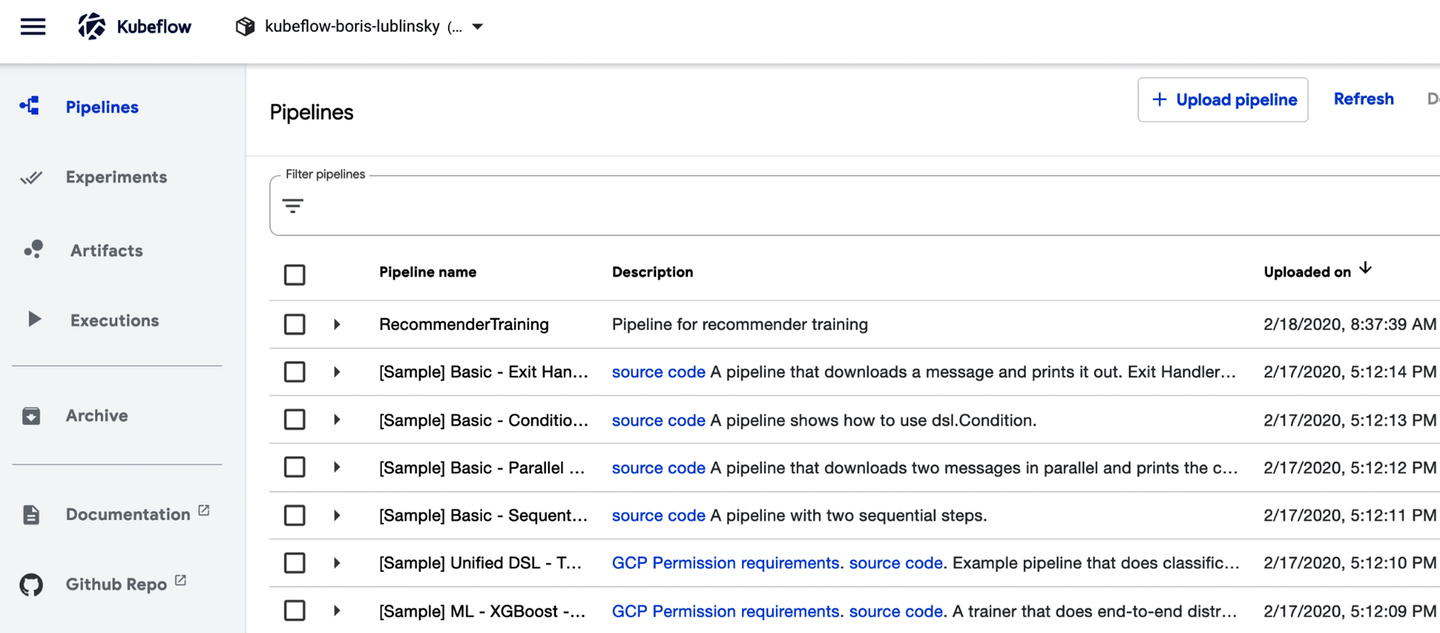
Figure 4-1. Kubeflow pipelines UI: prepackaged pipelines
Clicking a specific pipeline will show its execution graph or source, as seen in Figure 4-2.
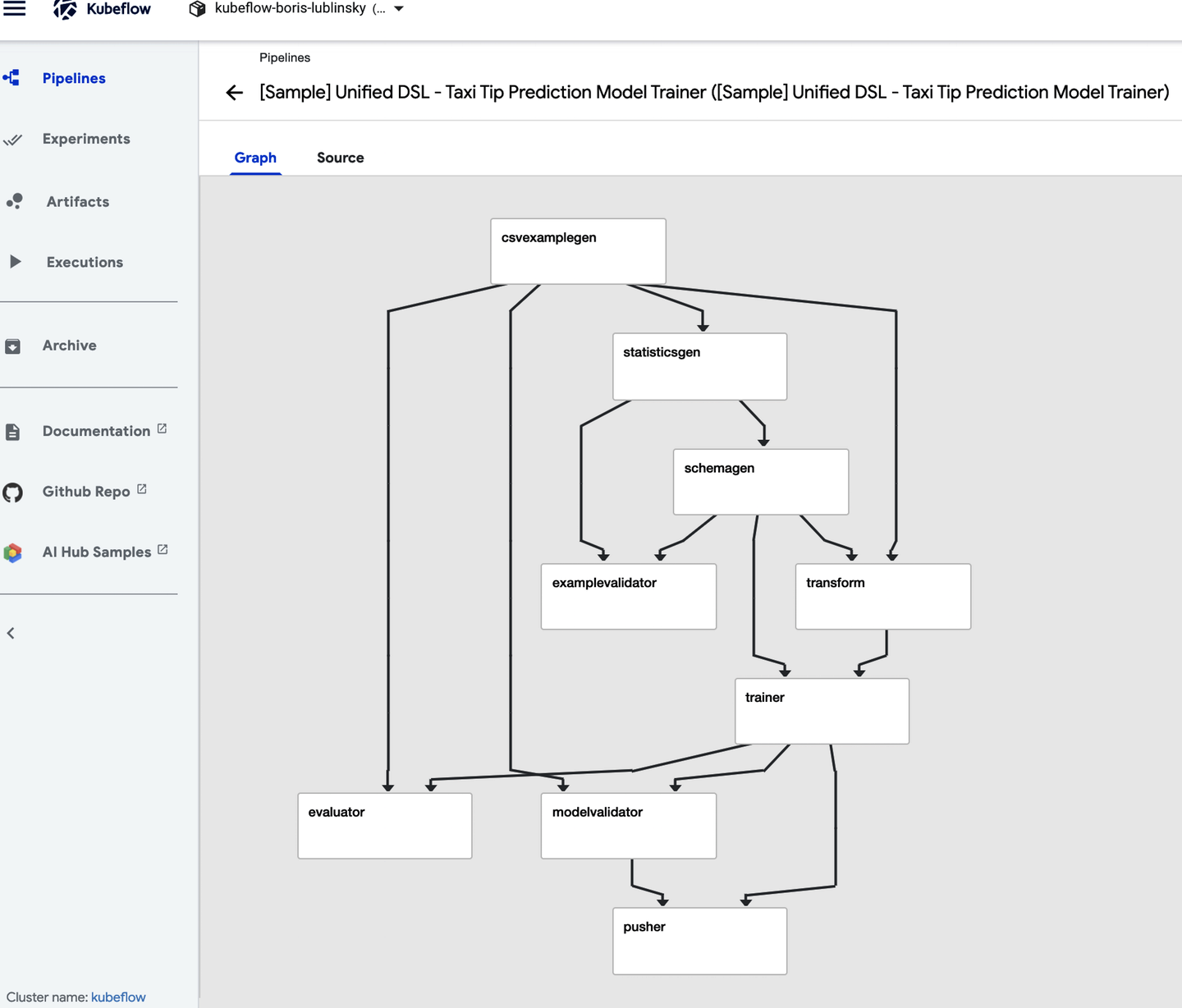
Figure 4-2. Kubeflow pipelines UI: pipeline graph view
Clicking the source tab will show the pipeline’s compiled code, which is an Argo YAML file (this is covered in more detail in “Argo: the Foundation of Pipelines”).
In this area you are welcome to experiment with running pipelines to get a better feel for their execution and the capabilities of the Pipelines UI.
To invoke a specific pipeline, simply click it; this will bring up Pipeline’s view as presented in Figure 4-3.
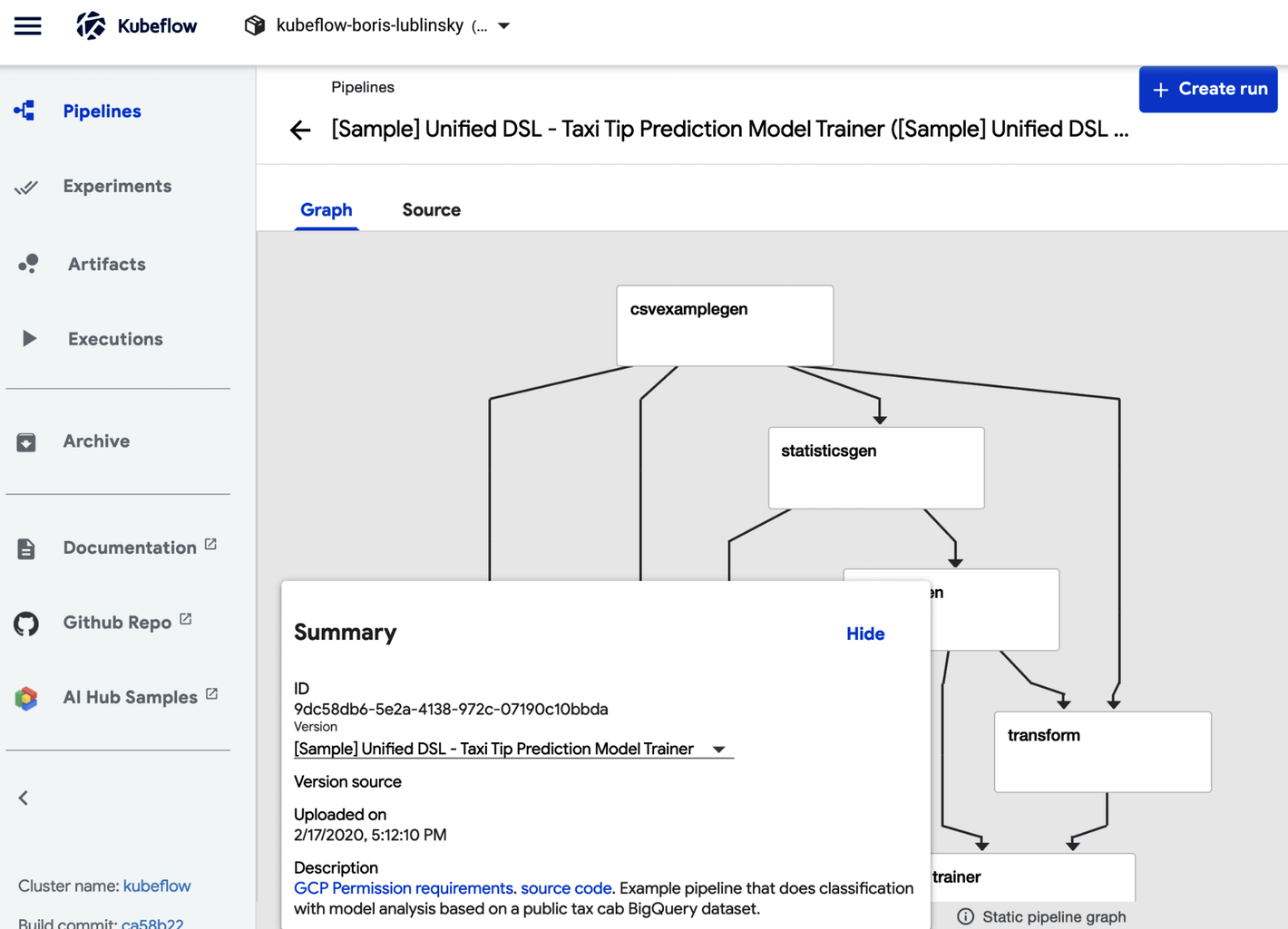
Figure 4-3. Kubeflow pipelines UI: pipeline view
To run the pipeline, click the “Create Run” button and follow the instructions on the screen.
Tip
When running a pipeline you must choose an experiment. Experiment here is just a convenience grouping for pipeline executions (runs). You can always use the “Default” experiment created by Kubeflow’s installation. Also, pick “One-off” for the Run type to execute the pipeline once. We will talk about recurring execution in “Running Pipelines on Schedule”.
Building a Simple Pipeline in Python
We have seen how to execute precompiled Kubeflow Pipelines, now let’s investigate how to author our own new pipelines. Kubeflow Pipelines are stored as YAML files executed by a program called Argo (see “Argo: the Foundation of Pipelines”). Thankfully, Kubeflow exposes a Python domain-specific language (DSL) for authoring pipelines. The DSL is a Pythonic representation of the operations performed in the ML workflow and built with ML workloads specifically in mind. The DSL also allows for some simple Python functions to be used as pipeline stages without you having to explicitly build a container.
Tip
The Chapter 4 examples can be found in the notebooks in this book’s GitHub repository.
A pipeline is, in its essence, a graph of container execution. In addition to specifying which containers should run in which order, it also allows the user to pass arguments to the entire pipeline and between participating containers.
For each container (when using the Python SDK), we must:
-
Create the container—either as a simple Python function, or with any Docker container (read more in Chapter 9).
-
Create an operation that references that container as well as the command line arguments, data mounts, and variable to pass the container.
-
Sequence the operations, defining which may happen in parallel and which must complete before moving on to a further step.1
-
Compile this pipeline, defined in Python, into a YAML file that Kubeflow Pipelines can consume.
Pipelines are a key feature of Kubeflow and you will see them again throughout the book. In this chapter we are going to show the simplest examples possible to illustrate the basic principles of Pipelines. This won’t feel like “machine learning” and that is by design.
For our first Kubeflow operation, we are going to use a technique known as lightweight Python functions. We should not, however, let the word lightweight deceive us. In a lightweight Python function, we define a Python function and then let Kubeflow take care of packaging that function into a container and creating an operation.
For the sake of simplicity, let’s declare the simplest of functions an echo. That is a function that takes a single input, an integer, and returns that input.
Let’s start by importing kfp and defining our function:
importkfpdefsimple_echo(i:int)->int:returni
Warning
Note that we use snake_case, not camelCase, for our function names. At the time of writing there exists a bug
(feature?) such that camel case names (for example: naming our function simpleEcho) will produce errors.
Next, we want to wrap our function simple_echo into a Kubeflow Pipeline operation. There’s a nice little
method to do this: kfp.components.func_to_container_op. This method returns a factory function with a strongly typed signature:
simpleStronglyTypedFunction=kfp.components.func_to_container_op(deadSimpleIntEchoFn)
When we create a pipeline in the next step, the factory function will construct a ContainerOp, which will run the original function (echo_fn) in a container:
foo=simpleStronglyTypedFunction(1)type(foo)Out[5]:kfp.dsl._container_op.ContainerOp
Tip
If your code can be accelerated by a GPU it is easy to mark a stage as using GPU resources; simply add .set_gpu_limit(NUM_GPUS) to your ContainerOp.
Now let’s sequence the ContainerOp(s) (there is only one) into a pipeline. This pipeline will take one parameter (the number we will echo). The pipeline also has a bit of metadata associated with it. While echoing numbers may be a trivial use of parameters, in real-world use cases you would include variables you might want to tune later such as hyperparameters for machine learning algorithms.
Finally, we compile our pipeline into a zipped YAML file, which we can then upload to the Pipelines UI.
@kfp.dsl.pipeline(name='Simple Echo',description='This is an echo pipeline. It echoes numbers.')defecho_pipeline(param_1:kfp.dsl.PipelineParam):my_step=simpleStronglyTypedFunction(i=param_1)kfp.compiler.Compiler().compile(echo_pipeline,'echo-pipeline.zip')
Tip
It is also possible to run the pipeline directly from the notebook, which we’ll do in the next example.
A pipeline with only one component is not very interesting. For our next example, we will customize the containers of our lightweight Python functions. We’ll create a new pipeline that installs and imports additional Python libraries, builds from a specified base image, and passes output between containers.
We are going to create a pipeline that divides a number by another number, and then adds a third number. First let’s create our simple add function, as shown in Example 4-1.
Example 4-1. A simple Python function
defadd(a:float,b:float)->float:'''Calculates sum of two arguments'''returna+badd_op=comp.func_to_container_op(add)
Next, let’s create a slightly more complex function. Additionally, let’s have this function require and import from a nonstandard Python library, numpy. This must be done within the function. That is because global imports from the notebook will not be packaged into the containers we create. Of course, it is also important to make sure that our container has the libraries we are importing installed.
To do that we’ll pass the specific container we want to use as our base image to .func_to_container(, as in Example 4-2.
Example 4-2. A less-simple Python function
fromtypingimportNamedTupledefmy_divmod(dividend:float,divisor:float)->\NamedTuple('MyDivmodOutput',[('quotient',float),('remainder',float)]):'''Divides two numbers and calculate the quotient and remainder'''#Imports inside a component function:importnumpyasnp#This function demonstrates how to use nested functions inside a# component function:defdivmod_helper(dividend,divisor):returnnp.divmod(dividend,divisor)(quotient,remainder)=divmod_helper(dividend,divisor)fromcollectionsimportnamedtupledivmod_output=namedtuple('MyDivmodOutput',['quotient','remainder'])returndivmod_output(quotient,remainder)divmod_op=comp.func_to_container_op(my_divmod,base_image='tensorflow/tensorflow:1.14.0-py3')

Importing libraries inside the function.

Nested functions inside lightweight Python functions are also OK.

Calling for a specific base container.
Now we will build a pipeline. The pipeline in Example 4-3 uses the functions defined previously, my_divmod and add, as stages.
Example 4-3. A simple pipeline
@dsl.pipeline(
   name='Calculation pipeline',
   description='A toy pipeline that performs arithmetic calculations.'
)
def calc_pipeline(
   a='a',
   b='7',
   c='17',
):
    #Passing pipeline parameter and a constant value as operation arguments
    add_task = add_op(a, 4) #Returns a dsl.ContainerOp class instance.

    #Passing a task output reference as operation arguments
    #For an operation with a single return value, the output
    # reference can be accessed using `task.output`
    # or `task.outputs['output_name']` syntax
    divmod_task = divmod_op(add_task.output, b)

    #For an operation with multiple return values, the output references
    # can be accessed using `task.outputs['output_name']` syntax
    result_task = add_op(divmod_task.outputs['quotient'], c)
Values being passed between containers. Order of operations is inferred from this.
Finally, we use the client to submit the pipeline for execution, which returns the links to execution and experiment.
Experiments group the executions together. You can also use kfp.compiler.Compiler().compile and upload the zip file as
in the first example if you prefer:
client=kfp.Client()#Specify pipeline argument values# arguments = {'a': '7', 'b': '8'} #whatever makes sense for new version#Submit a pipeline runclient.create_run_from_pipeline_func(calc_pipeline,arguments=arguments)
Following the link returned by create_run_from_pipeline_func, we can get to the execution web UI, which shows the
pipeline itself and intermediate results, as seen in Figure 4-4.
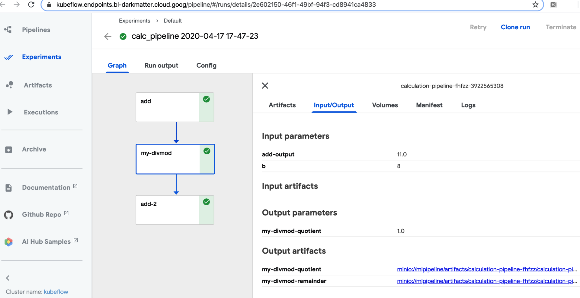
Figure 4-4. Pipeline execution
As we’ve seen, the lightweight in lightweight Python functions refers to the ease of making these steps in our process and not the power of the functions themselves. We can use custom imports, base images, and how to hand off small results between containers.
In the next section, we’ll show how to hand larger data files between containers by mounting volumes to the containers.
Storing Data Between Steps
In the previous example, the data passed between containers was small and of primitive types (such as numeric, string, list, and arrays). In practice however, we will likely be passing much larger data (for instance, entire datasets). In Kubeflow, there are two primary methods for doing this—persistent volumes inside the Kubernetes cluster, and cloud storage options (such as S3), though each method has inherent problems.
Persistent volumes abstract the storage layer. Depending on the vendor, persistent volumes can be slow with provisioning and have IO limits. Check to see if your vendor supports read-write-many storage classes, allowing for storage access by multiple pods, which is required for some types of parallelism. Storage classes can be one of the following.2
- ReadWriteOnce
-
The volume can be mounted as read-write by a single node.
- ReadOnlyMany
-
The volume can be mounted read-only by many nodes.
- ReadWriteMany
-
The volume can be mounted as read-write by many nodes.
Your system/cluster administrator may be able to add read-write-many support.3 Additionally, many cloud providers include their proprietary read-write-many implementations, see for example dynamic provisioning on GKE. but make sure to ask if there is a single node bottleneck.
Kubeflow Pipelines’ VolumeOp allows you to create an automatically managed persistent volume, as shown in Example 4-4. To add the volume to your operation you can just call add_pvolumes with a dictionary of mount points to volumes, e.g., download_data_op(year).add_pvolumes({"/data_processing": dvop.volume}).
Example 4-4. Mailing list data prep
dvop=dsl.VolumeOp(name="create_pvc",resource_name="my-pvc-2",size="5Gi",modes=dsl.VOLUME_MODE_RWO)
While less common in the Kubeflow examples, using an object storage solution, in some cases, may be more suitable. MinIO provides cloud native object storage by working either as a gateway to an existing object storage engine or on its own.4 We covered how to configure MinIO back in Chapter 3.
Kubeflow’s built-in file_output mechanism automatically transfers the specified local file into MinIO between pipeline steps for you. To use file_output, write your files locally in your container and specify the parameter in your ContainerOp, as shown in Example 4-5.
Example 4-5. File output example
fetch=kfp.dsl.ContainerOp(name='download',image='busybox',command=['sh','-c'],arguments=['sleep 1;''mkdir -p /tmp/data;''wget '+data_url+' -O /tmp/data/results.csv'],file_outputs={'downloaded':'/tmp/data'})# This expects a directory of inputs not just a single file
If you don’t want to use MinIO, you can also directly use your provider’s object storage, but this may compromise some portability.
The ability to mount data locally is an essential task in any machine learning pipeline. Here we have briefly outlined multiple methods and provided examples for each.
Introduction to Kubeflow Pipelines Components
Kubeflow Pipelines builds on Argo Workflows, an open source, container-native workflow engine for Kubernetes. In this section we will describe how Argo works, what it does, and how Kubeflow Pipeline supplements Argo to make it easier to use by data scientists.
Argo: the Foundation of Pipelines
Kubeflow installs all of the Argo components. Though having Argo installed on your computer is not necessary to use Kubeflow Pipelines, having the Argo command-line tool makes it easier to understand and debug your pipelines.
Tip
By default, Kubeflow configures Argo to use the Docker executor. If your platform does not support the Docker APIs, you need to switch your executor to a compatible one. This is done by changing the containerRuntimeExecutor value in the Argo params file. See Appendix A for details on the trade-offs. The majority of the examples in this book use the Docker executor but can be adapted to other executors.
On macOS, you can install Argo with Homebrew, as shown in Example 4-6.5
Example 4-6. Argo installation
#!/bin/bash# Download the binarycurl -sLO https://github.com/argoproj/argo/releases/download/v2.8.1/argo-linux-amd64# Make binary executablechmod +x argo-linux-amd64# Move binary to pathmv ./argo-linux-amd64 ~/bin/argo
You can verify your Argo installation by running the Argo examples with the command-line tool in the Kubeflow namespace: follow these Argo instructions.
When you run the Argo examples the pipelines are visible with the argo command, as in Example 4-7.
Example 4-7. Listing Argo executions
$ argo list -n kubeflow
NAME                STATUS      AGE   DURATION
loops-maps-4mxp5    Succeeded   30m   12s
hello-world-wsxbr   Succeeded   39m   15s
Since pipelines are implemented with Argo, you can use the same technique to check on them as well. You can also get information about specific workflow execution, as shown in Example 4-8.
Example 4-8. Getting Argo execution details
$argogethello-world-wsxbr-nkubeflowName:hello-world-wsxbrNamespace:kubeflowServiceAccount:defaultStatus:SucceededCreated:TueFeb1210:05:04-0600(2minutesago)Started:TueFeb1210:05:04-0600(2minutesago)Finished:TueFeb1210:05:23-0600(1minuteago)Duration:19secondsSTEPPODNAMEDURATIONMESSAGE✔hello-world-wsxbrhello-world-wsxbr18s
hello-world-wsxbris the name that we got usingargo list -n kubeflowabove. In your case the name will be different.
We can also view the execution logs by using the command in Example 4-9.
Example 4-9. Getting the log of Argo execution
$ argo logs hello-world-wsxbr -n kubeflowThis produces the result shown in Example 4-10.
Example 4-10. Argo execution log
< hello world >
 -------------
    \
     \
      \
		    ##        .
	      ## ## ##       ==
	   ## ## ## ##      ===
       /""""""""""""""""___/ ===
  ~~~ {~~ ~~~~ ~~~ ~~~~ ~~ ~ /  ===- ~~~
       \______ o          __/
	\    \        __/
	  \____\______/
You can also delete a specific workflow; see Example 4-11.
Example 4-11. Deleting Argo execution
$ argo delete hello-world-wsxbr -n kubeflowAlternatively, you can get pipeline execution information using the Argo UI, as seen in Figure 4-5.
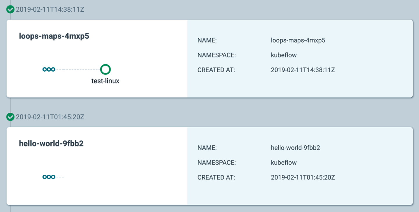
Figure 4-5. Argo UI for pipeline execution
You can also look at the details of the flow execution graph by clicking a specific workflow, as seen in Figure 4-6.
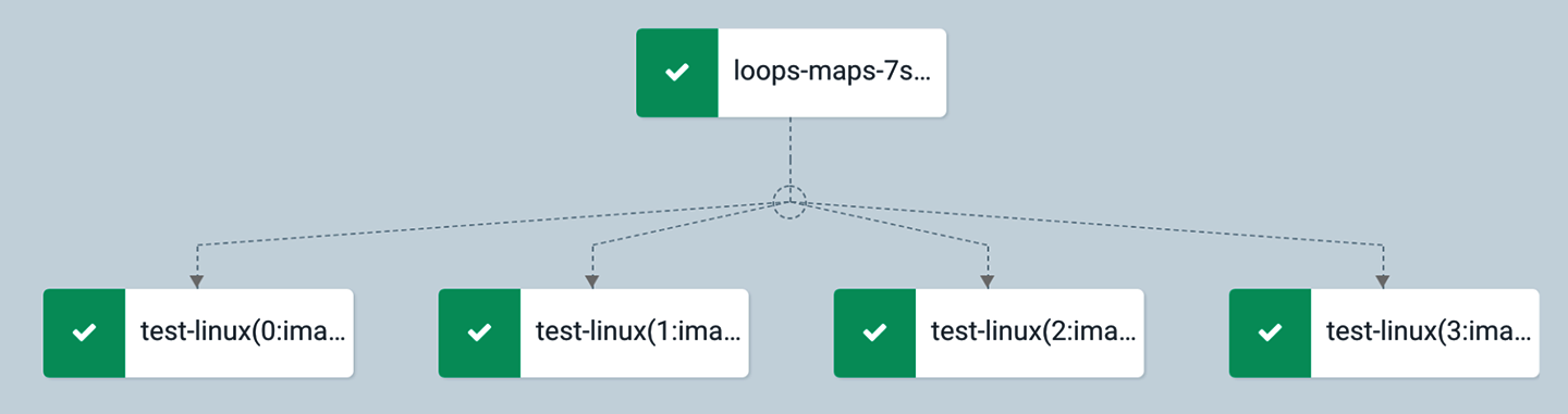
Figure 4-6. Argo UI execution graph
For any Kubeflow pipeline you run, you can also view that pipeline in the Argo CLI/UI. Note that because ML pipelines are using the Argo CRD, you can also see the result of the pipeline execution in the Argo UI (as in Figure 4-7).
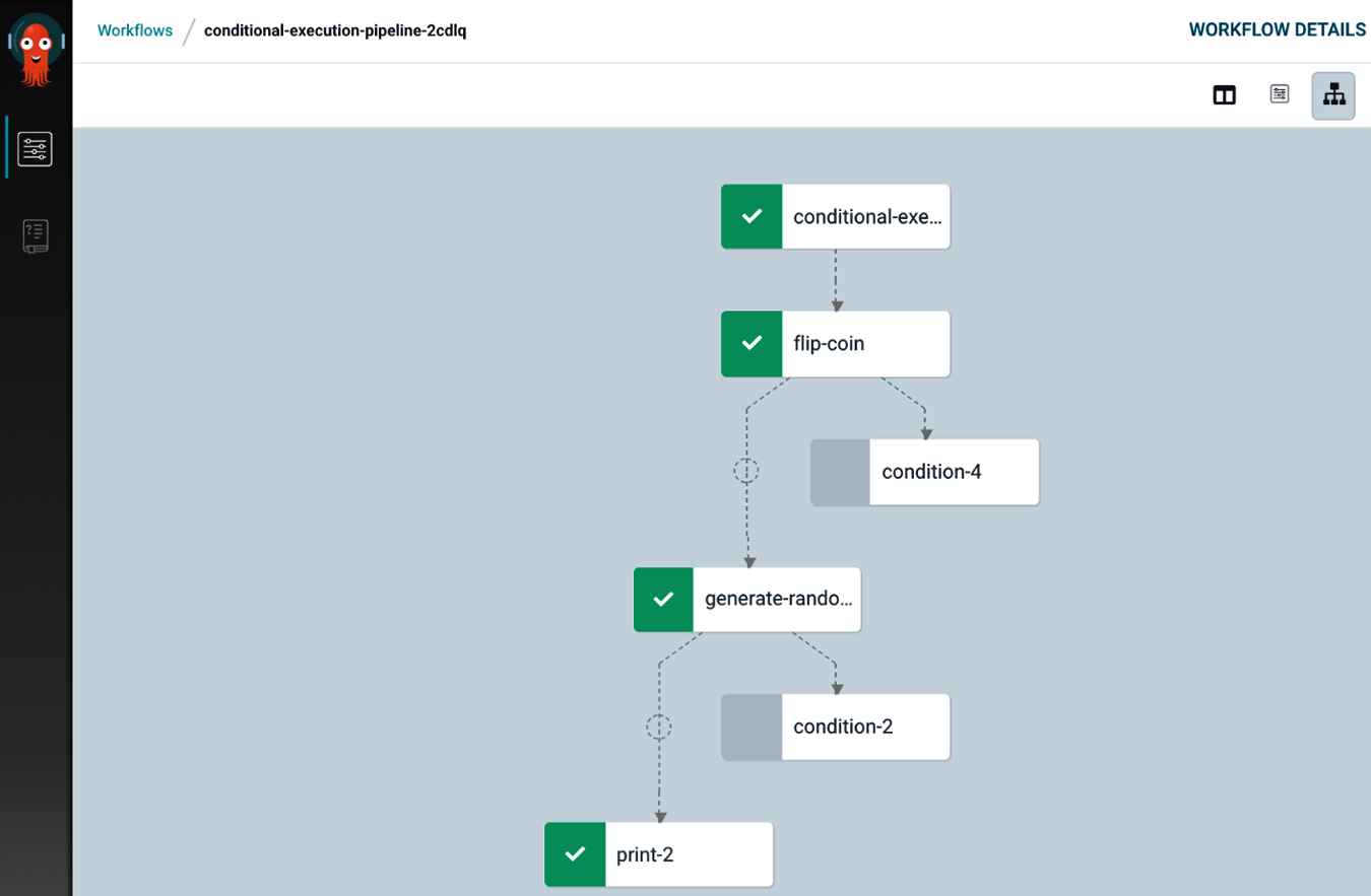
Figure 4-7. Viewing Kubeflow pipelines in Argo UI
Tip
Currently, the Kubeflow community is actively looking at alternative foundational technologies for running Kubeflow pipelines, one of which is Tekton. The paper by A. Singh et al., “Kubeflow Pipelines with Tekton”, gives “initial design, specifications, and code for enabling Kubeflow Pipelines to run on top of Tekton.” The basic idea here is to create an intermediate format that can be produced by pipelines and then executed using Argo, Tekton, or other runtimes. The initial code for this implementation is found in this Kubeflow GitHub repo.
What Kubeflow Pipelines Adds to Argo Workflow
Argo underlies the workflow execution; however, using it directly requires you to do awkward things. First, you must define your workflow in YAML, which can be difficult. Second, you must containerize your code, which can be tedious. The main advantage of KF Pipelines is that you can use Python APIs for defining/creating pipelines, which automates the generation of much of the YAML boilerplate for workflow definitions and is extremely friendly for data scientists/Python developers. Kubeflow Pipelines also has hooks that add building blocks for machine learning-specific components. These APIs not only generate the YAML but can also simplify container creation and resource usage. In addition to the APIs, Kubeflow adds a recurring scheduler and UI for configuration and execution.
Building a Pipeline Using Existing Images
Building pipeline stages directly from Python provides a straightforward entry point. It does limit our implementation to Python, though. Another feature of Kubeflow Pipelines is the ability to orchestrate the execution of a multilanguage implementation leveraging prebuilt Docker images (see Chapter 9).
In addition to our previous imports, we also want to import the Kubernetes client, which allows us to use Kubernetes functions directly from Python code (see Example 4-12).
Example 4-12. Exporting Kubernetes client
fromkubernetesimportclientask8s_client
Again, we create a client and experiment to run our pipeline. As mentioned earlier, experiments group the runs of pipelines. You can only create a given experiment once, so Example 4-13 shows how to either create a new experiment or use an existing one.
Example 4-13. Obtaining pipeline experiment
client=kfp.Client()exp=client.get_experiment(experiment_name='mdupdate')
Now we create our pipeline (Example 4-14). The images used need to be accessible, and we’re specifying the full names, so they resolve. Since these containers are prebuilt, we need to configure them for our pipeline.
The pre-built containers we are using have their storage configured by the MINIO_* environment variables. So we configure them to use our local MinIO install by calling add_env_variable.
In addition to the automatic dependencies created when passing parameters between stages, you can also specify that a
stage requires a previous stage with after. This is most useful when there is an external side effect, like updating a database.
Example 4-14. Example recommender pipeline
@dsl.pipeline(name='Recommender model update',description='Demonstrate usage of pipelines for multi-step model update')defrecommender_pipeline():# Load new datadata=dsl.ContainerOp(name='updatedata',image='lightbend/recommender-data-update-publisher:0.2')\.add_env_variable(k8s_client.V1EnvVar(name='MINIO_URL',value='http://minio-service.kubeflow.svc.cluster.local:9000'))\.add_env_variable(k8s_client.V1EnvVar(name='MINIO_KEY',value='minio'))\.add_env_variable(k8s_client.V1EnvVar(name='MINIO_SECRET',value='minio123'))# Train the modeltrain=dsl.ContainerOp(name='trainmodel',image='lightbend/ml-tf-recommender:0.2')\.add_env_variable(k8s_client.V1EnvVar(name='MINIO_URL',value='minio-service.kubeflow.svc.cluster.local:9000'))\.add_env_variable(k8s_client.V1EnvVar(name='MINIO_KEY',value='minio'))\.add_env_variable(k8s_client.V1EnvVar(name='MINIO_SECRET',value='minio123'))train.after(data)# Publish new modelpublish=dsl.ContainerOp(name='publishmodel',image='lightbend/recommender-model-publisher:0.2')\.add_env_variable(k8s_client.V1EnvVar(name='MINIO_URL',value='http://minio-service.kubeflow.svc.cluster.local:9000'))\.add_env_variable(k8s_client.V1EnvVar(name='MINIO_KEY',value='minio'))\.add_env_variable(k8s_client.V1EnvVar(name='MINIO_SECRET',value='minio123'))\.add_env_variable(k8s_client.V1EnvVar(name='KAFKA_BROKERS',value='cloudflow-kafka-brokers.cloudflow.svc.cluster.local:9092'))\.add_env_variable(k8s_client.V1EnvVar(name='DEFAULT_RECOMMENDER_URL',value='http://recommendermodelserver.kubeflow.svc.cluster.local:8501'))\.add_env_variable(k8s_client.V1EnvVar(name='ALTERNATIVE_RECOMMENDER_URL',value='http://recommendermodelserver1.kubeflow.svc.cluster.local:8501'))publish.after(train)
Since the pipeline definition is just code, you can make it more compact by using a loop to set the MinIO parameters instead of doing it on each stage.
As before, we need to compile the pipeline, either explicitly with compiler.Compiler().compile or implicitly with
create_run_from_pipeline_func. Now go ahead and run the pipeline (as in Figure 4-8).

Figure 4-8. Execution of recommender pipelines example
Kubeflow Pipeline Components
In addition to container operations which we’ve just discussed, Kubeflow Pipelines also exposes additional operations
with components. Components expose different Kubernetes resources or external operations (like dataproc). Kubeflow components allow developers to package machine learning tools while abstracting away the specifics on the containers or CRDs used.
We have used Kubeflow’s building blocks fairly directly, and we have used the func_to_container component.6
Some components, like func_to_container, are available as Python code and can be imported like normal. Other components are specified using Kubeflow’s component.yaml system and need to be loaded. In our opinion, the best way to work with Kubeflow components is to download a specific tag of the repo, allowing us to use load_component_from_file, as shown in Example 4-15.
Example 4-15. Pipeline release
wget https://github.com/kubeflow/pipelines/archive/0.2.5.tar.gz
tar -xvf 0.2.5.tar.gz
Warning
There is a load_component function that takes a component’s name and attempts to resolve it. We don’t recommend
using this function since it defaults to a search path that includes fetching, from Github, the master branch of the pipelines library, which is unstable.
We explore data preparation components in depth in the next chapter; however, let’s quickly look at a file-fetching component as an example. In our recommender example earlier in the chapter, we used a special prebuilt container to fetch our data since it was not already in a persistent volume. Instead, we can use the Kubeflow GCS component google-cloud/storage/download/ to download our data. Assuming you’ve downloaded the pipeline release as in Example 4-15, you can load the component with load_component_from_file as in Example 4-16.
Example 4-16. Load GCS download component
gcs_download_component=kfp.components.load_component_from_file("pipelines-0.2.5/components/google-cloud/storage/download/component.yaml")
When a component is loaded, it returns a function that produces a pipeline stage when called. Most components take parameters to configure their behavior. You can get a list of the components’ options by calling help on the loaded component, or looking at the component.yaml. The GCS download component requires us to configure what we are downloading
with gcs_path, shown in Example 4-17.
Example 4-17. Loading pipeline storage component from relative path and web link
dl_op=gcs_download_component(gcs_path="gs://ml-pipeline-playground/tensorflow-tfx-repo/tfx/components/testdata/external/csv")# Your path goes here
In Chapter 5, we explore more common Kubeflow pipeline components for data and feature preparation.
Advanced Topics in Pipelines
All of the examples that we have shown so far are purely sequential. There are also cases in which we need the ability to check conditions and change the behavior of the pipeline accordingly.
Conditional Execution of Pipeline Stages
Kubeflow Pipelines allows conditional executions via dsl.Condition. Let’s look at a very simple example, where, depending on the value of a variable, different calculations are executed.
A simple notebook implementing this example follows. It starts with the imports necessary for this, in Example 4-18.
Example 4-18. Importing required components
importkfpfromkfpimportdslfromkfp.componentsimportfunc_to_container_op,InputPath,OutputPath
Once the imports are in place, we can implement several simple functions, as shown in Example 4-19.
Example 4-19. Functions implementation
@func_to_container_opdefget_random_int_op(minimum:int,maximum:int)->int:"""Generate a random number between minimum and maximum (inclusive)."""importrandomresult=random.randint(minimum,maximum)(result)returnresult@func_to_container_opdefprocess_small_op(data:int):"""Process small numbers."""("Processing small result",data)return@func_to_container_opdefprocess_medium_op(data:int):"""Process medium numbers."""("Processing medium result",data)return@func_to_container_opdefprocess_large_op(data:int):"""Process large numbers."""("Processing large result",data)return
We implement all of the functions directly using Python (as in the previous example). The first function generates an integer between 0 and 100, and the next three constitute a simple skeleton for the actual processing. The pipeline is implemented as in Example 4-20.
Example 4-20. Pipeline implementation
@dsl.pipeline(name='Conditional execution pipeline',description='Shows how to use dsl.Condition().')defconditional_pipeline():number=get_random_int_op(0,100).outputwithdsl.Condition(number<10):process_small_op(number)withdsl.Condition(number>10andnumber<50):process_medium_op(number)withdsl.Condition(number>50):process_large_op(number)kfp.Client().create_run_from_pipeline_func(conditional_pipeline,arguments={})
Depending on the number we get here…
We will continue on to one of these operations.
Note here that we are specifying empty arguments—required parameter.
Finally, the execution graph, as shown in Figure 4-9.
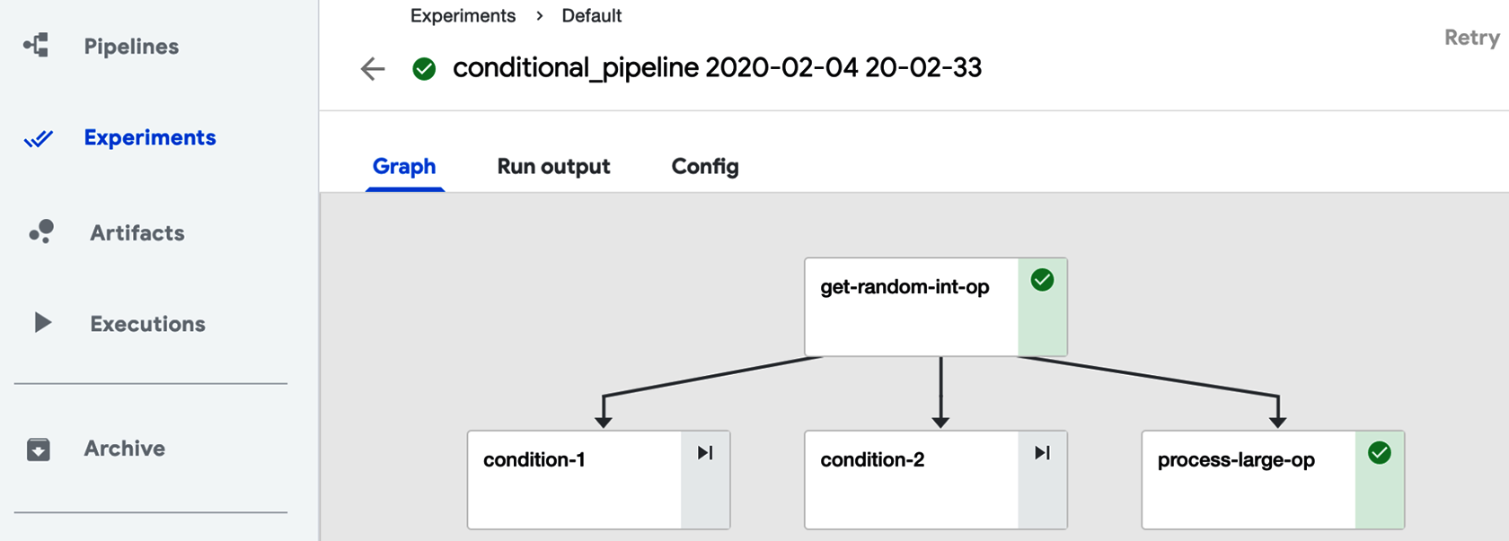
Figure 4-9. Execution of conditional pipelines example
From this graph, we can see that the pipeline really splits into three branches and process-large-op execution is selected in this run. To validate that this is correct, we look at the execution log, shown in Figure 4-10.
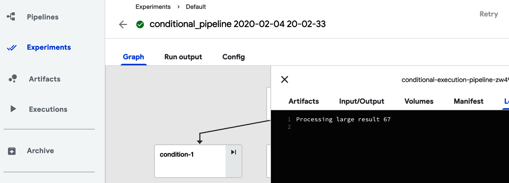
Figure 4-10. Viewing conditional pipeline log
Here we can see that the generated number is 67. This number is larger than 50, which means that the process_large_op branch should be executed.7
Running Pipelines on Schedule
We have run our pipeline manually. This is good for testing, but is often insufficient for production environments. Fortunately, you can run pipelines on a schedule, as described on thisKubeflow documentation page. First, you need to upload a pipeline definition and specify a description. When this is done, you can create a periodic run by creating a run and selecting a run type of “Recurring,” then following the instructions on the screen, as seen in Figure 4-11.
In this figure we are setting a pipeline to run every day.
Warning
When creating a periodic run we are specifying how often to run a pipeline, not when to run it. In the current implementation, the time of execution is defined by when the run is created. Once it is created, it is executed immediately and then executed with the defined frequency. If, for example, a daily run is created at 10 am, it will be executed at 10 am daily.
Setting periodic execution of pipelines is an important functionality, allowing you to completely automate pipeline execution.
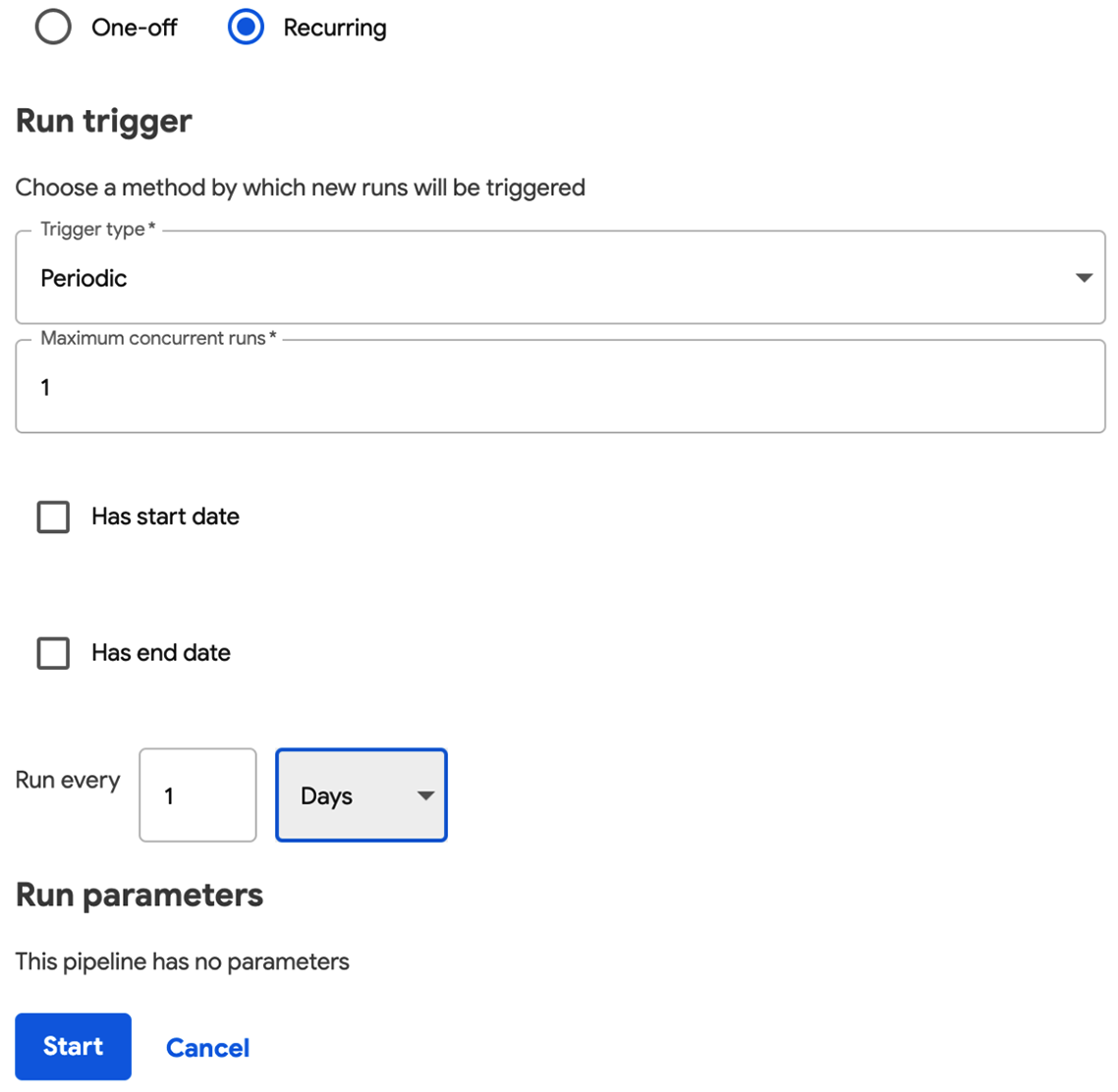
Figure 4-11. Setting up periodic execution of a pipeline
Conclusion
You should now have the basics of how to build, schedule, and run some simple pipelines. You also learned about the tools that pipelines use for when you need to debug. We showed how to integrate existing software into pipelines, how to implement conditional execution inside a pipeline, and how to run pipelines on a schedule.
In our next chapter, we look at how to use pipelines for data preparation with some examples.
1 This can often be automatically inferred when passing the result of one pipeline stage as the input to others. You can also specify additional dependencies manually.
2 Kubernetes persistent volumes can provide different access modes.
3 Generic read-write-many implementation is NFS server.
4 Usage of the cloud native access storage can be handy if you need to ensure portability of your solution across multiple cloud providers.
5 For installation of Argo Workflow on another OS, refer to these Argo instructions.
6 Many of the standard components are in this Kubeflow GitHub repo.
7 A slightly more complex example of conditional processing (with nested conditions) can be found in this GitHub site.
Get Kubeflow for Machine Learning now with the O’Reilly learning platform.
O’Reilly members experience books, live events, courses curated by job role, and more from O’Reilly and nearly 200 top publishers.

