Introducing MLOps

Chapter 4. Developing Models

Adrien Lavoillotte

Anyone who wants to be serious about MLOps needs to have at least a cursory understanding of the model development process, which is presented in Figure 4-1 as an element of the larger ML project life cycle. Depending on the situation, the model development process can range from quite simple to extremely complex, and it dictates the constraints of subsequent usage, monitoring, and maintenance of models.

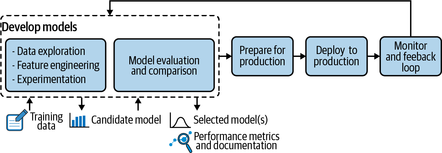
Figure 4-1. Model development highlighted in the larger context of the ML project life cycle

The implications of the data collection process on the rest of the model’s life is quite straightforward, and one easily sees how a model can become stale. For other parts of the model, the effects may be less obvious.

For example, take feature creation, where feeding a date to the model versus a flag indicating whether the day is a public holiday may make a big difference in performance, but also comes with significantly different constraints on updating the model. Or consider how the metrics used for evaluating and comparing models may enable automatic switching to the best possible version down the line, should the situation require it.

This chapter therefore covers the basics of model development, specifically in the context of MLOps, that is, how models might be built and developed in ways that make MLOps considerations easier to implement down the line.

What Is a Machine Learning Model?

Machine learning models are leveraged both in academia and in the real world (i.e., business contexts), so it’s important to distinguish what they represent in theory versus how they are implemented in practice. Let’s dive into both, building on what we’ve already seen in Chapter 3.

In Theory

A machine learning model is a projection of reality; that is, it’s a partial and approximate representation of some aspect (or aspects) of a real thing or process. Which aspects are represented often depends on what is available and useful. A machine learning model, once trained, boils down a mathematical formula that yields a result when fed some inputs—say, a probability estimation of some event happening or the estimated value of a raw number.

Machine learning models are based on statistical theory, and machine learning algorithms are the tools that build models from training data. Their goal is to find a synthetic representation of the data they are fed, and this data represents the world as it was at the time of collection. Therefore, machine learning models can be used to make predictions when the future looks like the past, because their synthetic representation is still valid.

Generalization Capacity

Machine learning models’ ability to accurately predict for cases that are not exactly like the input data is called their generalization capacity. Even when they yield outputs like horses with zebra stripes¹ that do not exist in training datasets, they do it by modeling a probability distribution that allows them to have this kind of surprising generalization capacity.

An often-used example for how machine learning models can predict and generalize is the price of a house. Of course, the selling price of a house will depend on too many factors too complex to model precisely, but getting close enough to be useful is not so difficult. The input data for that model may be things inherent to the house like surface area, number of bedrooms and bathrooms, year of construction, location, etc., but also other more contextual information like the state of the housing market at the time of sale, whether the seller is in a hurry, and so on. With complete enough historical data, and provided the market conditions do not change too much, an algorithm can compute a formula that provides a reasonable estimate.

Another frequent example is a health diagnosis or prediction that someone will develop a certain disease within a given timeframe. This kind of classification model often outputs the probability of some event, sometimes also with a confidence interval.

In Practice

A model is the set of parameters necessary to rebuild and apply the formula. It is usually stateless and deterministic (i.e., the same inputs always give the same outputs, with some exceptions; see “Online Learning”).

This includes the parameters of the end formula itself, but it also includes all the transformations to go from the input data that will be fed to the model to the end formula that will yield a value plus the possible derived data (like a classification or a decision). Given this description in practice, it usually does not make a difference whether the model is ML-based or not: it is just a computable mathematical function applied to the input data, one row at a time.

In the house price case, for instance, it may not be practical to gather enough pricing data for every zip code to get a model that’s accurate enough in all target locations. Instead, maybe the zip codes will be replaced with some derived inputs that are deemed to have the most influence on price—say, average income, population density, or proximity to some amenities. But since end users will continue to input the zip code and not these derived inputs, for all intents and purposes, all of this transformation is also part of the pricing model.

Outputs can also be richer than a single number. A system that detects fraud, for example, will often provide some kind of probability (and in some cases maybe also a confidence interval) rather than a binary answer. Depending on the acceptability of fraud and the cost of subsequent verification or denial of the transaction, it may be set up to only classify fraudulent instances where the probability reaches some fine-tuned threshold. Some models even include recommendations or decisions, such as which product to show a visitor to maximize spending or which treatment provides the most probable recovery.

All of these transformations and associated data are part of the model to some degree; however, this does not mean they are always bundled in a monolithic package, as one single artifact compiled together. This could quickly get unwieldy, and, in addition, some parts of this information come with varying constraints (different refresh rates, external sources, etc.).

Required Components

Building a machine learning model requires many components as outlined in Table 4-1.

Table 4-1. Required components of a machine learning model

ML component	Description
Training data	Training data is usually labeled for the prediction case with examples of what is being modeled (supervised learning). It might sound obvious, but it’s important to have good training data. An illustrative example of when this was not the case was data from damaged planes during World War II, which suffered from survivor bias and therefore was not good training data.
A performance metric	A performance metric is what the model being developed seeks to optimize. It should be chosen carefully to avoid unintended consequences, like the cobra effect (named for a famous anecdote, where a reward for dead cobras led some to breed them). For example, if 95% of the data has class A, optimizing for raw accuracy may produce a model that always predicts A and is 95% accurate.
ML algorithm	There are a variety of models that work in various ways and have different pros and cons. It is important to note that some algorithms are more suited to certain tasks than others, but their selection also depends on what needs to be prioritized: performance, stability, interpretability, computation cost, etc.
Hyperparameters	Hyperparameters are configurations for ML algorithms. The algorithm contains the basic formula, the parameters it learns are the operations and operands that make up this formula for that particular prediction task, and the hyperparameters are the ways that the algorithm may go to find these parameters. For example, in a decision tree (where data continues to be split in two according to what looks to be the best predictor in the subset that reached this path), one hyperparameter is the depth of the tree (i.e., the number of splits).
Evaluation dataset	When using labeled data, an evaluation dataset that is different from the training set will be required to evaluate how the model performs on unseen data (i.e., how well it can generalize).

The sheer number and complexity of each individual component is part of what can make good MLOps a challenging undertaking. But the complexity doesn’t stop here, as algorithm choice is yet another piece of the puzzle.

Different ML Algorithms, Different MLOps Challenges

What ML algorithms all have in common is that they model patterns in past data to make inferences, and the quality and relevance of this experience are the key factors in their effectiveness. Where they differ is that each style of algorithm has specific characteristics and presents different challenges in MLOps (outlined in Table 4-2).

Table 4-2. MLOps considerations by algorithm type

Algorithm type	Name	MLOps considerations
Linear	Linear regression	There is a tendency for overfitting.
	Logistic regression	There is a tendency for overfitting.
Tree-based	Decision tree	Can be unstable—small changes in data can lead to a large change in the structure of the optimal decision tree.
	Random forest	Predictions can be difficult to understand, which is challenging from a Responsible AI perspective. Random forest models can also be relatively slow to output predictions, which can present challenges for applications.
	Gradient boosting	Like random forest, predictions can be difficult to understand. Also, a small change in the feature or training set can create radical changes in the model.
Deep learning	Neural networks	In terms of interpretability, deep learning models are almost impossible to understand. Deep learning algorithms, including neural networks, are also extremely slow to train and require a lot of power (and data). Is it worth the resources, or would a simpler model work just as well?

Some ML algorithms can best support specific use cases, but governance considerations may also play a part in the choice of algorithm. In particular, highly regulated environments where decisions must be explained (e.g., financial services) cannot use opaque algorithms such as neural networks; rather, they have to favor simpler techniques, such as decision trees. In many use cases, it’s not so much a trade-off on performance but rather a trade-off on cost. That is, simpler techniques usually require more costly manual feature engineering to reach the same level of performance as more complex techniques.

Computing Power

When talking about components of machine learning model development, it’s impossible to ignore computing power. Some say planes fly thanks to human ingenuity, but it’s also thanks to a lot of fuel. This holds true with machine learning as well: its development is inversely proportional to the cost of computing power.

From hand-computed linear regression of the early twentieth century to today’s largest deep learning models, new algorithms arose when the required computing power became available. For example, mainstream algorithms like random forest and gradient boosting both require a computing power that was expensive 20 years ago.

In exchange, they brought an ease of use that considerably lowered the cost of developing ML models, thus putting new use cases within the reach of the average organization. The decrease in the cost of data also helped, but it was not the first driver: very few algorithms leverage big data technology in which both data and computation are distributed over a large number of computers; rather, most of them still operate with all the training data in memory.

Data Exploration

When data scientists or analysts consider data sources to train a model, they need to first get a grasp of what that data looks like. Even a model trained using the most effective algorithm is only as good as its training data. At this stage, a number of issues can prevent all or part of the data from being useful, including incompleteness, inaccuracy, inconsistency, etc.

Examples of such processes can include:

• Documenting how the data was collected and what assumptions were already made

• Looking at summarizing statistics of the data: What is the domain of each column? Are there some rows with missing values? Obvious mistakes? Strange outliers? No outliers at all?

• Taking a closer look at the distribution of the data

• Cleaning, filling, reshaping, filtering, clipping, sampling, etc.

• Checking correlations between the different columns, running statistical tests on some subpopulations, fitting distribution curves

• Comparing that data to other data or models in the literature: Is there some usual information that seems to be missing? Is this data comparably distributed?

Of course, domain knowledge is required to make informed decisions during this exploration. Some oddities may be hard to spot without specific insight, and assumptions made can have consequences that are not obvious to the untrained eye. Industrial sensor data is a good example: unless the data scientist is also a mechanical engineer or expert in the equipment, they might not know what constitutes normal versus strange outliers for a particular machine.

Feature Engineering and Selection

Features are how data is presented to a model, serving to inform that model on things it may not infer by itself. This table provides examples of how features may be engineered:

Feature engineering category	Description
Derivatives	Infer new information from existing information—e.g., what day of the week is this date?
Enrichment	Add new external information—e.g., is this day a public holiday?
Encoding	Present the same information differently—e.g., day of the week or weekday versus weekend.
Combination	Link features together—e.g., the size of the backlog might need to be weighted by the complexity of the different items in it.

For instance, in trying to estimate the potential duration of a business process given the current backlog, if one of the inputs is a date, it is pretty common to derive the corresponding day of the week or how far ahead the next public holiday is from that date. If the business serves multiple locations that observe different business calendars, that information may also be important.

Another example, to follow up on the house pricing scenario from the previous section, would be using average income and population density, which ideally allows the model to better generalize and train on more diverse data than trying to segment by area (i.e., zip code).

Feature Engineering Techniques

A whole market exists for such complementary data that extends far beyond the open data that public institutions and companies share. Some services provide direct enrichment that can save a lot of time and effort.

There are, however, many cases when information that data scientists need for their models is not available. In this case, there are techniques like impact coding, whereby data scientists replace a modality by the average value of the target for that modality, thus allowing the model to benefit from data in a similar range (at the cost of some information loss).

Ultimately, most ML algorithms require a table of numbers as input, each row representing a sample, and all samples coming from the same dataset. When the input data is not tabular, data scientists can use other tricks to transform it.

The most common one is one-hot encoding. For example, a feature that can take three values (e.g., Raspberry, Blueberry, and Strawberry) is transformed into three features that can take only two values—yes or no (e.g., Raspberry yes/no, Blueberry yes/no, Strawberry yes/no).

Text or image inputs, on the other hand, require more complex engineering. Deep learning has recently revolutionized this field by providing models that transform images and text into tables of numbers that are usable by ML algorithms. These tables are called embeddings, and they allow data scientists to perform transfer learning because they can be used in domains on which they were not trained.

Transfer Learning

Transfer learning is the technique of using information gained from solving one problem in solving a different problem. Transfer learning can be used to significantly accelerate learning of second or subsequent tasks, and it is very popular in deep learning, where the resources needed to train models can be enormous.

For example, even if a particular deep learning model was trained on images that did not contain any forks, it may give a useful embedding to be used by a model that is trained to detect them, because a fork is an object, and that model was trained to detect similar human-made objects.

How Feature Selection Impacts MLOps Strategy

When it comes to feature creation and selection, the question of how much and when to stop comes up regularly. Adding more features may produce a more accurate model, achieve more fairness when splitting into more precise groups, or compensate for some other useful missing information. However, it also comes with downsides, all of which can have a significant impact on MLOps strategies down the line:

• The model can become more and more expensive to compute.

• More features require more inputs and more maintenance down the line.

• More features mean a loss of some stability.

• The sheer number of features can raise privacy concerns.

Automated feature selection can help by using heuristics to estimate how critical some features will be for the predictive performance of the model. For instance, one can look at the correlation with the target variable or quickly train a simple model on a representative subset of the data and then look at which features are the strongest predictors.

Which inputs to use, how to encode them, how they interact or interfere with each other—such decisions require a certain understanding of the inner workings of the ML algorithm. The good news is that some of this can be partly automated, e.g., by using tools such as Auto-sklearn or AutoML applications that cross-reference features against a given target to estimate which features, derivatives, or combinations are likely to yield the best results, leaving out all the features that would probably not make that much of a difference.

Other choices still require human intervention, such as deciding whether to try to collect additional information that might improve the model. Spending time to build business-friendly features will often improve the final performance and ease the adoption by end users, as model explanations are likely to be simpler. It can also reduce modeling debt, allowing data scientists to understand the main prediction drivers and ensure that they are robust. Of course, there are trade-offs to consider between the cost of time spent to understand the model and the expected value, as well as risks associated with the model’s use.

Feature Stores

Feature factories, or feature stores, are repositories of different features associated with business entities that are created and stored in a central location for easier reuse. They usually combine an offline part (slower, but potentially more powerful) and an online part (quicker and more useful for real-time needs), making sure they remain consistent with each other.

Given how time-consuming feature engineering is for data scientists, feature stores have huge potential to free up their time for even more valuable tasks. Machine learning is still often the “high-interest credit card of technical debt”. Reversing this will require huge efficiency gains in the data-to-model-to-production process and in the MLOps process, and feature stores are one way to get there.

The bottom line is that when building models, the process of engineering and selecting features, like many other ML model components, is a delicate balance between considering MLOps components and performance.

Experimentation

Experimentation takes place throughout the entire model development process, and usually every important decision or assumption comes with at least some experiment or previous research to justify it. Experimentation can take many shapes, from building full-fledged predictive ML models to doing statistical tests or charting data. Goals of experimentation include:

• Assessing how useful or how good of a model can be built given the elements outlined in Table 4-1. (The next section will cover model evaluation and comparison in more detail.)

• Finding the best modeling parameters (algorithms, hyperparameters, feature preprocessing, etc.).

• Tuning the bias/variance trade-off for a given training cost to fit that definition of “best.”

• Finding a balance between model improvement and improved computation costs. (Since there’s always room for improvement, how good is good enough?)

Bias and Variance

A high bias model (also known as underfitting) fails to discover some of the rules that could have been learned from the training data, possibly because of reductive assumptions making the model overly simplistic.

A high variance model (or overfitting) sees patterns in noise and seeks to predict every single variation, resulting in a complex model that does not generalize well beyond its training data.

When experimenting, data scientists need to be able to quickly iterate through all the possibilities for each of the model building blocks outlined in Table 4-1. Fortunately, there are tools to do all of this semiautomatically, where you only need to define what should be tested (the space of possibilities) depending on prior knowledge (what makes sense) and the constraints (e.g., computation, budget).

Some tools allow for even more automation, for instance by offering stratified model training. For example, say the business wants to predict customer demand for products to optimize inventory, but behavior varies a lot from one store to the next. Stratified modeling consists of training one model per store that can be better optimized for each store rather than a model that tries to predict in all stores.

Trying all combinations of every possible hyperparameter, feature handling, etc., quickly becomes untraceable. Therefore, it is useful to define a time and/or computation budget for experiments as well as an acceptability threshold for usefulness of the model (more on that notion in the next section).

Notably, all or part of this process may need to be repeated every time anything in the situation changes (including whenever the data and/or problem constraints change significantly; see “Drift Detection in Practice”). Ultimately, this means that all experiments that informed the final decisions data scientists made to arrive at the model as well as all the assumptions and conclusions along the way may need to be rerun and reexamined.

Fortunately, more and more data science and machine learning platforms allow for automating these workflows not only on the first run, but also to preserve all the processing operations for repeatability. Some also allow for the use of version control and experimental branch spin-off to test theories and then merge, discard, or keep them (see “Version Management and Reproducibility”).

Evaluating and Comparing Models

George E. P. Box, a twentieth century British statistician, once said that all models are wrong, but some are useful. In other words, a model should not aim to be perfect, but it should pass the bar of “good enough to be useful” while keeping an eye on the uncanny valley—typically a model that looks like it’s doing a good job but does a bad (or catastrophic) job for a specific subset of cases (say, an underrepresented population).

With this in mind, it’s important to evaluate a model in context and have some ability to compare it to what existed before the model—whether a previous model or a rules-based process—to get an idea of what the outcome would be if the current model or decision process were replaced by the new one.

A model with an absolute performance that could technically be considered disappointing can still possibly enhance an existing situation. For instance, having a slightly more accurate forecast of demand for a certain product or service may result in huge cost-savings.

Conversely, a model that gets a perfect score is suspicious, as most problems have noise in the data that’s at least somewhat hard to predict. A perfect or nearly-perfect score may be a sign that there is a leak in the data (i.e., that the target to be predicted is also in the input data or that an input feature is very correlated to the target but, practically, available only once the target is known) or that the model overfits the training data and will not generalize well.

Choosing Evaluation Metrics

Choosing the proper metric by which to evaluate and compare different models for a given problem can lead to very different models (think of the cobra effect mentioned in Table 4-1). A simple example: accuracy is often used for automated classification problems but is rarely the best fit when the classes are unbalanced (i.e., when one of the outcomes is very unlikely compared to the other). In a binary classification problem where the positive class (i.e., the one that is interesting to predict because its prediction triggers an action) is rare, say 5% of occurrences, a model that constantly predicts the negative class is therefore 95% accurate, while also utterly useless.

Unfortunately, there is no one-size-fits-all metric. You need to pick one that matches the problem at hand, which means understanding the limits and trade-offs of the metric (the mathematics side) and their impact on the optimization of the model (the business side).

To get an idea of how well a model will generalize, that metric should be evaluated on a part of the data that was not used for the model’s training (a holdout dataset), a method called cross-testing. There can be multiple steps where some data is held for evaluation and the rest is used for training or optimizing, such as metric evaluation or hyperparameter optimization. There are different strategies as well, not necessarily just a simple split. In k-fold cross-validation, for example, data scientists rotate the parts that they hold out to evaluate and train multiple times. This multiplies the training time but gives an idea of the stability of the metric.

With a simple split, the holdout dataset can consist of the most recent records instead of randomly chosen ones. Indeed, as models are usually used for future predictions, it is likely that assessing them as if they were used for prediction on the most recent data leads to more realistic estimations. In addition, it allows one to assess whether the data drifted between the training and the holdout dataset (see “Drift Detection in Practice” for more details).

As an example, Figure 4-2 shows a scheme in which a test dataset is a holdout (in gray) in order to perform the evaluation. The remaining data is split into three parts to find the best hyperparameter combination by training the model three times with a given combination on each of the blue datasets, and validating its performance on their respective green datasets. The gray dataset is used only once with the best hyperparameter combination, while the other datasets are used with all of them.

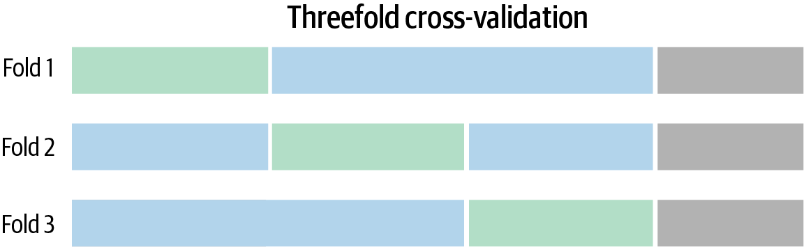
Figure 4-2. An example of dataset split for model evaluation

Oftentimes, data scientists want to periodically retrain models with the same algorithms, hyperparameters, features, etc., but on more recent data. Naturally, the next step is to compare the two models and see how the new version fares. But it’s also important to make sure all previous assumptions still hold: that the problem hasn’t fundamentally shifted, that the modeling choices made previously still fit the data, etc. This is more specifically part of performance and drift monitoring (find more details on this in Chapter 7).

Cross-Checking Model Behavior

Beyond the raw metrics, when evaluating a model, it’s critical to understand how it will behave. Depending on the impact of the model’s predictions, decisions, or classifications, a more or less deep understanding may be required. For example, data scientists should take reasonable steps (with respect to that impact) to ensure that the model is not actively harmful: a model that would predict that all patients need to be checked by a doctor may score high in terms of raw prevention, but not so much on realistic resource allocation.

Examples of these reasonable steps include:

• Cross-checking different metrics (and not only the ones on which the model was initially optimized)

• Checking how the model reacts to different inputs—e.g., plot the average prediction (or probability for classification models) for different values of some inputs and see whether there are oddities or extreme variability

• Splitting one particular dimension and checking the difference in behavior and metrics across different subpopulations—e.g., is the error rate the same for males and females?

These kinds of global analyses should not be understood as causality, just as correlation. They do not necessarily imply a specific causal relationship between some variables and an outcome; they merely show how the model sees that relationship. In other words, the model should be used with care for what-if analysis. If one feature value is changed, the model prediction is likely to be wrong if the new feature value has never been seen in the training dataset or if it has never been seen in combination with the values of the other features in this dataset.

When comparing models, those different aspects should be accessible to data scientists, who need to be able to go deeper than a single metric. That means the full environment (interactive tooling, data, etc.) needs to be available for all models, ideally allowing for comparison from all angles and between all components. For example, for drift, the comparison might use the same settings but different data, while for modeling performance, it might use the same data but different settings.

Impact of Responsible AI on Modeling

Depending on the situation (and sometimes depending on the industry or sector of the business), on top of a general understanding of model behavior, data scientists may also need models’ individual predictions to be explainable, including having an idea of what specific features pushed the prediction one way or the other. Sometimes predictions may be very different for a specific record than on average. Popular methods to compute individual prediction explanations include Shapley value (the average marginal contribution of a feature value across all possible coalitions) and individual conditional expectation (ICE) computations, which show the dependence between the target functions and features of interest.

For example, the measured level of a specific hormone could generally push a model to predict someone has a health issue, but for a pregnant woman, that level makes the model infer she is at no such risk. Some legal frameworks mandate some kind of explainability for decisions made by a model that have consequences on humans, like recommending a loan to be denied. “Element 2: Bias” discusses this topic in detail.

Note that the notion of explainability has several dimensions. In particular, deep learning networks are sometimes called black-box models because of their complexity (though when reading the model coefficients, a model is fully specified, and it is usually a conceptually remarkably simple formula, but a very large formula that becomes impossible to intuitively apprehend). Conversely, global and local explanation tools—such as partial dependence plots or Shapley value computations—give some insights but arguably do not make the model intuitive. To actually communicate a rigorous and intuitive understanding of what exactly the model is doing, limiting the model complexity is required.

Fairness requirements can also have dimensioning constraints on model development. Consider this theoretical example to better understand what is at stake when it comes to bias: a US-based organization regularly hires people who do the same types of jobs. Data scientists could train a model to predict the workers’ performance according to various characteristics, and people would then be hired based on the probability that they would be high-performing workers.

Though this seems like a simple problem, unfortunately, it’s fraught with pitfalls. To make this problem completely hypothetical and to detach it from the complexities and problems of the real world, let’s say everyone in the working population belongs to one of two groups: Weequay or Togruta.

For this hypothetical example, let’s claim that a far larger population of Weequay attend university. Off the bat, there would be an initial bias in favor of Weequay (amplified by the fact they would have been able to develop their skills through years of experience).

As a result, there would not only be more Weequay than Togruta in the pool of applicants, but Weequay applicants would tend to be more qualified. The employer has to hire 10 people during the month to come. What should it do?

• As an equal opportunity employer, it should ensure the fairness of its recruitment process as it controls it. That means in mathematical terms, for each applicant and all things being equal, being hired (or not) should not depend on their group affiliation (in this case, Weequay or Togruta). However, this results in bias in and of itself, as Weequay are more qualified. Note that “all things being equal” can be interpreted in various ways, but the usual interpretation is that the organization is likely not considered accountable for processes it does not control.

• The employer may also have to avoid disparate impact, that is, practices in employment that adversely affect one group of people of a protected characteristic more than another. Disparate impact is assessed on subpopulations and not on individuals; practically, it assesses whether proportionally speaking, the company has hired as many Weequay as Togruta. Once again, the target proportions may be those of the applicants or those of the general population, though the former is more likely, as again, the organization can’t be accountable for biases in processes out of its control.

The two objectives are mutually exclusive. In this scenario, equal opportunity would lead to hiring 60% (or more) Weequay and 40% (or fewer) Togruta. As a result, the process has a disparate impact on the two populations, because the hiring rates are different.

Conversely, if the process is corrected so that 40% of people hired are Togruta to avoid disparate impact, it means that some rejected Weequay applicants will have been predicted as more qualified than some accepted Togruta applicants (contradicting the equal opportunity assertion).

There needs to be a trade-off—the law sometimes referred to as the 80% rule. In this example, it would mean that the hiring rate of Togruta should be equal to or larger than 80% of the hiring rate of Weequay. In this example, it means that it would be OK to hire up to 65% Weequay.

The point here is that defining these objectives cannot be a decision made by data scientists alone. But even once the objectives are defined, the implementation itself may also be problematic:

• Without any indications, data scientists naturally try to build equal opportunity models because they correspond to models of the world as it is. Most of the tools data scientists employ also try to achieve this because it is the most mathematically sound option. Yet some ways to achieve this goal may be unlawful. For example, the data scientist may choose to implement two independent models: one for Weequay and one for Togruta. This could be a reasonable way to address the biases induced by a training dataset in which Weequay are overrepresented, but it would induce a disparate treatment of the two that could be considered discriminatory.

• To let data scientists use their tools in the way they were designed (i.e., to model the world as it is), they may decide to post-process the predictions so that they fit with the organization’s vision of the world as it should be. The simplest way of doing this is to choose a higher threshold for Weequay than for Togruta. The gap between them will adjust the trade-off between “equal opportunity” and “equal impact”; however, it may still be considered discriminatory because of the disparate treatment.

Data scientists are unlikely to be able to sort this problem out alone (see “Key Elements of Responsible AI” for a broader view on the subject). This simple example illustrates the complexity of the subject, which may be even more complex given that there may be many protected attributes, and the fact that bias is as much a business question as a technical question.

Consequently, the solution heavily depends on the context. For instance, this example of Weequay and Togruta is representative of processes that give access to privileges. The situation is different if the process has negative impacts on the user (like fraud prediction that leads to transaction rejection) or is neutral (like disease prediction).

Version Management and Reproducibility

Discussing the evaluation and comparison of models (for fairness as discussed immediately before, but also a host of other factors) necessarily brings up the idea of version control and the reproducibility of different model versions. With data scientists building, testing, and iterating on several versions of models, they need to be able to keep all the versions straight.

Version management and reproducibility address two different needs:

• During the experimentation phase, data scientists may find themselves going back and forth on different decisions, trying out different combinations, and reverting when they don’t produce the desired results. That means having the ability to go back to different “branches” of the experiments—for example, restoring a previous state of a project when the experimentation process led to a dead end.

• Data scientists or others (auditors, managers, etc.) may need to be able to replay the computations that led to model deployment for an audit team several years after the experimentation was first done.

Versioning has arguably been somewhat solved when everything is code-based, with source version control technology. Modern data processing platforms typically offer similar capabilities for data transformation pipelines, model configuration, etc. Merging several parts is, of course, less straightforward than merging code that diverged, but the basic need is to be able to go back to some specific experiment, if only to be able to copy its settings to replicate them in another branch.

Another very important property of a model is reproducibility. After a lot of experiments and tweaking, data scientists may arrive at a model that fits the bill. But after that, operationalization necessitates model reproduction not only in another environment, but also possibly from a different starting point. Repeatability also makes debugging much easier (sometimes even simply possible). To this end, all facets of the model need to be documented and reusable, including:

Assumptions

When a data scientist makes decisions and assumptions about the problem at hand, its scope, the data, etc., they should all be explicit and logged so that they can be checked against any new information down the line.

Randomness

A lot of ML algorithms and processes, such as sampling, make use of pseudo-random numbers. Being able to precisely reproduce an experiment, such as for debugging, means to have control over that pseudo-randomness, most often by controlling the “seed” of the generator (i.e., the same generator initialized with the same seed would yield the same sequence of pseudo-random numbers).

Data

To get repeatability, the same data must be available. This can sometimes be tricky because the storage capacity required to version data can be prohibitive depending on the rate of update and quantity. Also, branching on data does not yet have as rich an ecosystem of tools as branching on code.

Settings

This one is a given: all processing that has been done must be reproducible with the same settings.

Results

While developers use merging tools to compare and merge different text file versions, data scientists need to be able to compare in-depth analysis of models (from confusion matrices to partial dependence plots) to obtain models that satisfy the requirements.

Implementation

Ever-so-slightly different implementations of the same model can actually yield different models, enough to change the predictions on some close calls. And the more sophisticated the model, the higher the chances that these discrepancies happen. On the other hand, scoring a dataset in bulk with a model comes with different constraints than scoring a single record live in an API, so different implementations may sometimes be warranted for the same model. But when debugging and comparing, data scientists need to keep the possible differences in mind.

Environment

Given all the steps covered in this chapter, it’s clear that a model is not just its algorithm and parameters. From the data preparation to the scoring implementation, including feature selection, feature encoding, enrichment, etc., the environment in which several of those steps run may be more or less implicitly tied to the results. For instance, a slightly different version of a Python package involved in one step may change the results in ways that can be hard to predict. Preferably, data scientists should make sure that the runtime environment is also repeatable. Given the pace at which ML is evolving, this might require techniques that freeze the computation environments.

Fortunately, part of the underlying documentation tasks associated with versioning and reproducibility can be automated, and the use of an integrated platform for design and deployment can greatly decrease the reproducibility costs by ensuring structured information transfer.

Clearly, while maybe not the sexiest part of model development, version management and reproducibility are critical to building machine learning efforts in real-world organizational settings where governance—including audits—matters.

Closing Thoughts

Model development is one of the most critical and consequential steps of MLOps. The many technical questions that are necessarily answered during this phase have big repercussions on all aspects of the MLOps process throughout the life of the models. Therefore, exposure, transparency, and collaboration are crucial to long-term success.

The model development stage is also the one that has been practiced the most by profiles like data scientists and, in the pre-MLOps world, often represents the whole ML effort, yielding a model that will then be used as is (with all its consequences and limitations).

¹ CycleGAN is the implementation of recent research by Jun-Yan Zhu, Taesung Park, Phillip Isola, and Alexei A. Efros.