Hands-On Generative AI with Transformers and Diffusion Models

Chapter 4. Diffusion Models

The field of image generation became widely popular with Ian Goodfellow’s introduction of Generative Adversarial Nets (GANs) in 2014. The key ideas of GANs led to a big family of models that could quickly generate high-quality images. However, despite their success, GANs posed challenges, requiring many parameters and help to generalize effectively. These limitations sparked parallel research endeavors, leading to the exploration of diffusion models—a class of models that would redefine the landscape of high-quality, flexible image generation.

In late 2020, a little-known class of models called diffusion models began causing a stir in the ML world. Researchers figured out how to use these diffusion models to generate higher-quality images than those produced by GANs. A flurry of papers followed, proposing improvements and modifications that pushed the quality up even further. By late 2021, models like GLIDE showcased incredible results on text-to-image tasks. Just a few months later, these models had entered the mainstream with tools like DALL·E 2 and Stable Diffusion. These models made it easy for anyone to generate images just by typing in a text description of what they wanted to see.

In this chapter, we will dig into how these models work. We’ll outline the key insights that make them so powerful, generate images with existing models to get a feel for how they work, and then train our own to deepen this understanding further. The field is still rapidly evolving, but the topics covered here should give you a solid foundation to build on, which will be extended further in Chapters 5, 7, and 8.

The high-level idea of diffusion models is that they receive images blurred with noise and learn to denoise them, outputting a clear image. When diffusion models are trained, the dataset contains images with different amounts of noise (even when the input is pure noise). In inference, we can begin with pure noise, and the model will generate an image that matches the training distribution. The model does multiple iterations to accomplish this, correcting itself and leading to impressively high-quality generations.

The Key Insight: Iterative Refinement

So, what is it that makes diffusion models so powerful? Previous techniques, such as VAEs or GANs, generate their final output via a single forward pass of the model. This means the model must get everything right on the first try. If it makes a mistake, it can’t go back and fix it. Diffusion models, on the other hand, generate their output by iterating over many steps.¹ This iterative refinement allows the model to correct mistakes in previous steps and gradually improve the output. To illustrate this, Figure 4-1 shows an example of a diffusion model in action.

Figure 4-1. Progressive denoising process

We can load a pretrained diffusion model using the Hugging Face diffusers library. The library provides a high-level pipeline that can be used to create images directly. We’ll load the ddpm-celebahq-256 model, one of the first shared diffusion models for image generation. This model was trained with the CelebA-HQ dataset, a then-popular dataset of high-quality images of celebrities, so it will generate images that look like they came from that dataset. We’ll use this model to generate an image from noise:

import torch
from diffusers import DDPMPipeline

from genaibook.core import get_device

# Set the device to use our GPU or CPU
device = get_device()

# Load the pipeline
image_pipe = DDPMPipeline.from_pretrained("google/ddpm-celebahq-256")
image_pipe.to(device)

# Sample an image
image_pipe().images[0]

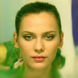
The pipeline does not show us what happens under the hood, so let’s dive into its internals. If you run the code, you will notice that generation took 1,000 steps. This diffusion pipeline has to go through 1,000 refinement steps (and forward passes) to get to the final image. This is one of the major drawbacks of the vanilla diffusion models compared to the GANs—they require many steps to generate high-quality images, making the models slow at inference time.

We can re-create this sampling process step-by-step to understand better what is happening under the hood. At the beginning of the diffusion process, we initialize our sample x with a batch of four random images (in other words, we sample some random noise). We’ll run 30 steps to progressively denoise the input images and end up with a sample from the real distribution.

Let’s generate some images! On the left side of the following image, you can see the input at a given step (beginning with the random noise). You can see the model’s prediction for the final images on the right. The results of the first row are not particularly good. Instead of jumping right to that final predicted image in a given diffusion step, we only modify the input x (shown on the left) by a small amount in the direction of the prediction. We then feed this new, slightly better x through the model again for the next step, hopefully resulting in a slightly improved prediction, which can be used to update x a little more, and so on. With enough steps, the model can produce some impressively realistic images:

from genaibook.core import plot_noise_and_denoise

# The random starting point is a batch of 4 images
# Each image is 3-channel (RGB) 256x256 pixel image
image = torch.randn(4, 3, 256, 256).to(device)

# Set the specific number of diffusion steps
image_pipe.scheduler.set_timesteps(num_inference_steps=30)

# Loop through the sampling timesteps
for i, t in enumerate(image_pipe.scheduler.timesteps):
    # Get the prediction given the current sample x and the timestep t
    # As we're running inference, we don't need to calculate gradients,
    # so we can use torch.inference_mode().
    with torch.inference_mode():
        # We need to pass in the timestep t so that the model knows what
        # timestep it's currently at. We'll learn more about this in the
        # coming sections.
        noise_pred = image_pipe.unet(image, t)["sample"]

    # Calculate what the updated x should look like with the scheduler
    scheduler_output = image_pipe.scheduler.step(noise_pred, t, image)

    # Update x
    image = scheduler_output.prev_sample

    # Occasionally display both x and the predicted denoised images
    if i % 10 == 0 or i == len(image_pipe.scheduler.timesteps) - 1:
        plot_noise_and_denoise(scheduler_output, i)

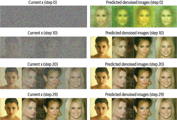
Don’t worry if that chunk of code looks intimidating—we’ll explain how this all works throughout this chapter. Focus on the idea for now.

This core idea of learning how to iteratively refine a noisy input can be applied to a wide range of tasks. This chapter will focus on unconditional image generation, generating images that resemble the training data distribution. For example, we can train an unconditional image-generation model with a dataset of butterflies so that it can also generate new, high-quality images. This model would not be able to create images different from the distribution of its training dataset, so don’t expect it to generate dinosaurs.

In Chapter 5, we’ll do a deep dive into diffusion models conditioned on text, but we can do many other things. Diffusion models have been applied to audio, video, text, 3D objects, protein structures, and other domains. While most implementations use some variant of the denoising approach we’ll cover here, emerging approaches that apply different types of “corruption” (always combined with iterative refinement) may move the field beyond the current focus on denoising diffusion.

Training a Diffusion Model

In this section, we’re going to train a diffusion model from scratch to gain a better understanding of how they work. We’ll start by using components from the diffusers library. As the chapter progresses, we’ll gradually demystify how each component works. Training a diffusion model is relatively straightforward compared to other generative models. To train a model, we repeatedly do the following:

1. Load some images from the training data.

2. Add noise in different amounts. Remember, we want the model to do a good job estimating how to “fix” (denoise) both extremely noisy images and images that are close to perfect, so we want a dataset with diverse amounts of noise.

3. Feed the noisy versions of the inputs into the model.

4. Evaluate how well the model does at denoising these inputs.

5. Use this information to update the model weights.

To generate new images with a trained model, we begin with a completely random input and repeatedly feed it through the model, updating the input on each iteration by a small amount based on the model prediction. As we’ll see, several sampling methods streamline this process to generate good images with as few steps as possible.

The Data

For this example, we’ll use a dataset of images from the Hugging Face Hub—specifically, a collection of 1,000 butterfly pictures.² Later on, in “Project Time: Train Your Diffusion Model”, you will see how to use your own data. Let’s load the butterflies dataset:

from datasets import load_dataset

dataset = load_dataset("huggan/smithsonian_butterflies_subset", split="train")

We must prepare the data before using it to train a model. Images are typically represented as a grid of pixels. Unlike in the previous chapter, where we used grayscale images, these images are in color. Each pixel is represented with color values between 0 and 255 for each of the three color channels (red, green, and blue). To process these and make them ready for training, we do the following:

1. Resize them to a fixed size. This is necessary because the model expects all images to have the same dimensions.

2. (Optional) Add some augmentation by randomly flipping them horizontally, making the model more robust and allowing us to train with more data. Augmentation (Figure 4-2) is a common practice in Computer Vision tasks, as it helps the model generalize better to unseen data. Flipping is just one technique of augmentation with image data. Other techniques are translating, scaling, and rotating.

   

   Figure 4-2. Augmentation creates more data from the training dataset, improving generalization

3. Convert them to a PyTorch tensor (representing the color values as floats between 0 and 1). Model inputs must always be formatted as multidimensional matrices, or tensors.

4. Normalize them to have a mean of 0, with values between –1 and 1. This is a common practice in training deep learning models, as it helps the model learn faster and more effectively.

We can define these transformations by using torchvision.transforms:³

from torchvision import transforms

image_size = 64

# Define transformations
preprocess = transforms.Compose(
    [
        transforms.Resize((image_size, image_size)),  # Resize
        transforms.RandomHorizontalFlip(),  # Randomly flip (data augmentation)
        transforms.ToTensor(),  # Convert to tensor (0, 1)
        transforms.Normalize([0.5], [0.5]),  # Map to (-1, 1)
    ]
)

The datasets library provides a convenient method, set_transform(), which allows us to specify transformations that will be applied on the fly as the data is used. Finally, we can wrap the dataset with a DataLoader, a loading utility that makes it easy to iterate over batches of data, simplifying our training code:

def transform(examples):
    examples = [preprocess(image) for image in examples["image"]]
    return {"images": examples}


dataset.set_transform(transform)
batch_size = 16

train_dataloader = torch.utils.data.DataLoader(
    dataset, batch_size=batch_size, shuffle=True
)

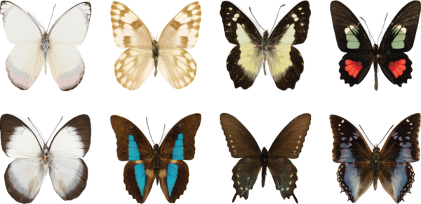
We can check that this worked by loading a batch and inspecting the images. Here’s an example batch from the training set:⁴

from genaibook.core import show_images

batch = next(iter(train_dataloader))

# When we normalized, we mapped (0, 1) to (-1, 1)
# Now we map back to (0, 1) for display
show_images(batch["images"][:8] * 0.5 + 0.5)

Adding Noise

How do we gradually corrupt our data? The most common approach is to add noise to the images. We will add different amounts of noise to the training data, as the goal is to train a robust model to denoise no matter how much noise is in the input. The amount of noise we add is controlled by a noise schedule, which is a critical aspect of diffusion models. Different papers and approaches tackle this in different ways.

For now, let’s explore one common approach in action based on the DDPM paper. In diffusers, adding noise is handled by a class called a Scheduler, which takes in a batch of images and a list of timesteps and determines how to create the noisy versions of those images. We’ll explore the math behind this later in the chapter, but for now, let’s see how it works in practice. The following code snippet applies increasingly larger amounts of noise to each one of the input images:

from diffusers import DDPMScheduler

# We'll learn about beta_start and beta_end in the next sections
scheduler = DDPMScheduler(
    num_train_timesteps=1000, beta_start=0.001, beta_end=0.02
)

# Create a tensor with 8 evenly spaced values from 0 to 999
timesteps = torch.linspace(0, 999, 8).long()

# We load 8 images from the dataset and
# add increasing amounts of noise to them
x = batch["images"][:8]
noise = torch.rand_like(x)
noised_x = scheduler.add_noise(x, noise, timesteps)
show_images((noised_x * 0.5 + 0.5).clip(0, 1))

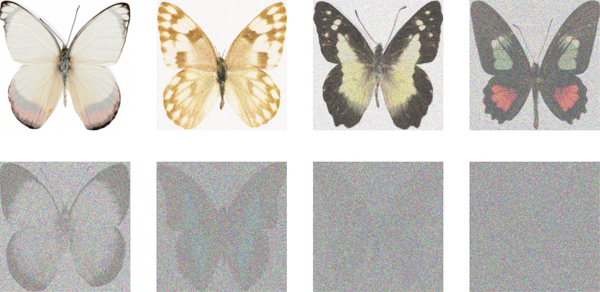
During training, we’ll pick the timesteps at random. The scheduler takes some parameters (beta_start and beta_end), which it uses to determine how much noise should be present for a given timestep. We will cover schedulers in more detail in “In Depth: Noise Schedules”.

The UNet

The UNet is a CNN invented for tasks such as image segmentation, where the desired output has the same shape as the input. For example, UNets are used in medical imaging to segment different anatomical structures.

As shown in Figure 4-3, the UNet consists of a series of downsampling layers that reduce the spatial size of the input, followed by a series of upsampling layers that increase the spatial extent of the input again. The downsampling layers are typically followed by skip connections that connect the downsampling layers’ outputs to the upsampling layers’ inputs. This allows the upsampling layers to incorporate finer details from earlier layers, preserving important high-resolution information during the denoising process.

The UNet architecture used in the diffusers library is more advanced than the original UNet proposed in 2015, with additions like attention and residual blocks. We’ll take a closer look later, but the key idea here is that it can take in an input and produce a prediction that is the same shape. In diffusion models, the input can be a noisy image, and the output can be the predicted noise. With this information, we can now denoise the input image.

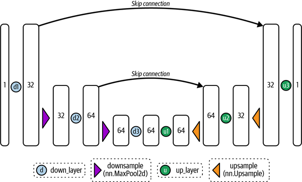
Figure 4-3. Architecture of a simplified UNet

Here’s how we might create a UNet and feed our batch of noisy images through it:

from diffusers import UNet2DModel

model = UNet2DModel(
    in_channels=3,  # 3 channels for RGB images
    sample_size=64,  # Specify our input size
    # The number of channels per block affects the model size
    block_out_channels=(64, 128, 256, 512),
    down_block_types=(
        "DownBlock2D",
        "DownBlock2D",
        "AttnDownBlock2D",
        "AttnDownBlock2D",
    ),
    up_block_types=("AttnUpBlock2D", "AttnUpBlock2D", "UpBlock2D", "UpBlock2D"),
).to(device)

# Pass a batch of data through to make sure it works
with torch.inference_mode():
    out = model(noised_x.to(device), timestep=timesteps.to(device)).sample

print(noised_x.shape)
print(out.shape)

torch.Size([8, 3, 64, 64])
torch.Size([8, 3, 64, 64])

Note that the output is the same shape as the input, which is exactly what we want.

Training

Now that we have our data and model ready, let’s train it. For each training step, we do the following:

1. Load a batch of images.

2. Add noise to the images. The amount of noise added depends on a specified number of timesteps: the more timesteps, the more noise. As mentioned, we want our model to denoise images with little noise and images with lots of noise. To achieve this, we’ll add random amounts of noise, so we’ll pick a random number of timesteps.

3. Feed the noisy images into the model.

4. Calculate the loss using MSE. MSE is a common loss function for regression tasks, including the UNet model’s noise prediction. It measures the average squared difference between predicted and true values, penalizing larger errors more. In the UNet model, MSE is calculated between predicted and actual noise, helping the model generate more realistic images by minimizing the loss. This is called the noise or epsilon objective.

5. Backpropagate the loss and update the model weights with the optimizer.

Here’s what all of that looks like in code. Training will take a while, so this is a great moment to pause, review the chapter’s content, or get some food:

from torch.nn import functional as F

num_epochs = 50  # How many runs through the data should we do?
lr = 1e-4  # What learning rate should we use
optimizer = torch.optim.AdamW(model.parameters(), lr=lr)
losses = []  # Somewhere to store the loss values for later plotting

# Train the model (this takes a while)
for epoch in range(num_epochs):
    for batch in train_dataloader:
        # Load the input images
        clean_images = batch["images"].to(device)

        # Sample noise to add to the images
        noise = torch.randn(clean_images.shape).to(device)

        # Sample a random timestep for each image
        timesteps = torch.randint(
            0,
            scheduler.config.num_train_timesteps,
            (clean_images.shape[0],),
            device=device,
        ).long()

        # Add noise to the clean images according
        # to the noise magnitude at each timestep
        noisy_images = scheduler.add_noise(clean_images, noise, timesteps)

        # Get the model prediction for the noise
        # The model also uses the timestep as an input
        # for additional conditioning
        noise_pred = model(noisy_images, timesteps, return_dict=False)[0]

        # Compare the prediction with the actual noise
        loss = F.mse_loss(noise_pred, noise)

        # Store the loss for later plotting
        losses.append(loss.item())

        # Update the model parameters with the optimizer based on this loss
        loss.backward()
        optimizer.step()
        optimizer.zero_grad()

Now that the model is trained, let’s plot the training loss:

from matplotlib import pyplot as plt

plt.subplots(1, 2, figsize=(12, 4))

plt.subplot(1, 2, 1)
plt.plot(losses)
plt.title("Training loss")
plt.xlabel("Training step")

plt.subplot(1, 2, 2)
plt.plot(range(400, len(losses)), losses[400:])
plt.title("Training loss from step 400")
plt.xlabel("Training step");

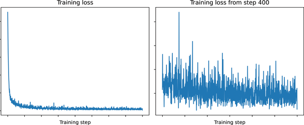
The loss curve on the left shows all the steps, while that on the right skips the first 400 steps. The loss curve trends downward as the model learns to denoise the images. The curve is somewhat noisy—the loss is not very stable. This is because each iteration uses different numbers of noising time steps. It is hard to tell whether this model will be good at generating samples by looking at the MSE of the noise predictions, so let’s move on to the next section and see how well it does.

Sampling

Now that we have a model, let’s do inference and generate some images. The diffusers library uses the idea of pipelines to bundle together all the components needed to generate samples with a diffusion model. We can use a pipeline to test the UNet we just trained; a few generations are shown as follows:⁵

pipeline = DDPMPipeline(unet=model, scheduler=scheduler)
ims = pipeline(batch_size=4).images
show_images(ims, nrows=1)

Offloading the job of creating samples to the pipeline doesn’t show us what is going on under the hood. So, let’s do a simple sampling loop showing how the model gradually refines the input image based on the code in the pipeline’s call() method:

# Random starting point (4 random images):
sample = torch.randn(4, 3, 64, 64).to(device)

for t in scheduler.timesteps:
    # Get the model prediction
    with torch.inference_mode():
        noise_pred = model(sample, t)["sample"]

    # Update sample with step
    sample = scheduler.step(noise_pred, t, sample).prev_sample

show_images(sample.clip(-1, 1) * 0.5 + 0.5, nrows=1)

This is the same code we used at the beginning of the chapter to illustrate the idea of iterative refinement, but now you better understand what is happening here. If you look at the implementation of the DDPMPipeline in the diffusers library, you’ll see that the logic closely resembles our implementation in the previous snippet.

We start with a completely random input, which the model then refines in a series of steps. Each step is a small update to the input based on the model’s prediction for the noise at that timestep. We’re still abstracting away some complexity behind the call to pipeline.scheduler.step(); later, we will dive deeper into different sampling methods and how they work.

Evaluation

Evaluating generative models is complex—it’s a subjective task in nature. For example, given an input prompt “image of a cat with sunglasses”, there are many potential correct generations. A common approach is to combine qualitative evaluation (e.g., by having humans compare generations) and quantitative metrics, which provide a framework for evaluation but don’t necessarily correspond to high image quality.

Fréchet Inception Distance (FID) scores can evaluate generative model performance. FID scores compare how similar two image datasets are. Using a pretrained neural network (an example is shown in Figure 4-4), they measure how closely generated samples match real samples by comparing statistics between feature maps extracted from both datasets. The lower the score, the better the quality and realism of generated images produced by a given model. FID scores are popular because of their ability to provide an “objective” comparison metric for different types of generative networks without relying on human judgment.

Figure 4-4. CNN network used to extract feature maps from images

As convenient as FID scores are, there are important caveats to be aware of (which might be true for other evaluation metrics as well):

• FID scores are designed to compare two distributions. Because of this, it assumes that we have access to a source dataset for comparison. A second issue is that you cannot calculate the FID score of a single generation. If we have one image, there’s no way to calculate its FID score.

• The FID score for a given model depends on the number of samples used to calculate it, so when comparing models, we need to make sure both reported scores are calculated using the same number of samples. The common practice is to use 50,000 samples for this purpose, although to save time, you may evaluate a smaller number during development and do the complete evaluation only after you’re ready to publish the results.

• The FID can be sensitive to many factors. For example, a different number of inference steps will lead to a very different FID. The scheduler (DDPM in this case) will also affect the FID.

• When calculating the FID, images are resized to 299 × 299 images. This makes it less useful as a metric for extremely low- or high-resolution images. There are also minor differences between how resizing is handled by different deep learning frameworks, which can result in slight differences in the FID score.

• The network used as a feature extractor for FID is typically a model trained on the ImageNet classification task.⁶ When generating images in a different domain, the features learned by this model may be less useful. A more accurate approach is to first train a classification network on domain-specific data, making comparing scores between different papers and techniques harder. For now, the ImageNet model is the standard choice.

• If you save generated samples for later evaluation, the format and compression can affect the FID score. Avoid low-quality JPEG images where possible.

Even if you account for all these caveats, FID scores are just a rough measure of quality and do not perfectly capture the nuances of what makes images look more “real.” The evaluation of generative models is an active research area. Standard metrics like Kernel Inception Distance (KID) and Inception Score share similar issues with FID. So, use these metrics to get an idea of how one model performs relative to another, but also look at the actual images generated by each model to get a better sense of how they compare.

Image quality, as measured by FID or KID, is only one of the metrics we can use to evaluate the performance of text-to-image models. Efforts such as Holistic Evaluation of Text-to-Image Models (HEIM) attempt to take into account additional desirable characteristics of text-to-image models, such as prompt adherence, originality, reasoning capabilities, multilingualism, absence of bias and toxicity, and others.

Human preference is still the gold standard for quality in what is ultimately a fairly subjective field. For example, the Parti Prompts dataset contains 1,600 prompts of varying difficulties and categories and allows comparing text-to-image models such as the ones we’ll explore in Chapter 5.⁷

In Depth: Noise Schedules

In the preceding training example, one of the steps was to “add noise in different amounts.” We achieved this by picking a random timestep between 0 and 1,000 and then relying on the scheduler to add the appropriate amount of noise. Likewise, during inference, we again relied on the scheduler to tell us which timesteps to use and how to move from one to the next, given the model predictions. Choosing how much noise to add is a crucial design decision that can drastically affect the performance of a given model. In this section, we’ll see why this is the case and explore different approaches used in practice.

Why Add Noise?

At the start of this chapter, we said that the key idea behind diffusion models is that of iterative refinement. During training, we corrupt an input by different amounts. During inference, we begin with a maximally corrupted input (that is, a pure noise image) and iteratively decorrupt it, expecting to end up with a nice final result eventually.

So far, we’ve focused on one specific kind of corruption: adding Gaussian noise. Gaussian noise is a type of noise that follows a normal distribution, which as we saw in Chapter 3, has most values around the mean and fewer values as we get further away.⁸ One reason for this focus is the theoretical underpinnings of diffusion models, which assume the use of Gaussian noise—if we use a different corruption method, we are no longer technically doing diffusion.

However, the Cold Diffusion paper demonstrated that we do not necessarily need to constrain ourselves to this method just for theoretical convenience. The authors showed (Figure 4-5) that a diffusion model–like approach works for many corruption methods. That means that rather than using noise, we can use other image transformations. For example, models such as Muse, MaskGIT, and Paella have used random token masking or replacement as equivalent corruption methods.

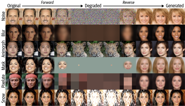
Figure 4-5. The general principles of diffusion work for other types of corruption, not just Gaussian noise (adapted from an image in the Cold Diffusion paper)

Nonetheless, adding noise remains the most popular approach for several reasons:

• We can easily control the amount of noise added, giving a smooth transition from “perfect” to “completely corrupted.” This is not the case for something like reducing the resolution of an image, which may result in “discrete” transitions.

• We can have many valid random starting points for inference, unlike some methods, which may have only a limited number of possible initial (fully corrupted) states, such as a completely black image or a single-pixel image.

So, for now, we’ll add noise as our corruption method. Next, let’s explore how we add noise to our images.

Starting Simple

We have some images, x, and we’d like to add some random noise to them. We generate pure Gaussian noise of the same dimensions as the input images with torch.rand_like():

x = next(iter(train_dataloader))["images"][:8]
noise = torch.rand_like(x)

One way we could add varying amounts of noise is to linearly interpolate (“lerp” for short) between the images and the noise by some amount. This gives us a function that smoothly transitions from the original image x to pure noise as the amount varies from 0 to 1:

def corrupt(x, noise, amount):
    # Reshape amount so it works correctly with the original data
    amount = amount.view(-1, 1, 1, 1)  # make sure it's broadcastable

    # Blend the original data and noise based on the amount
    return (
        x * (1 - amount) + noise * amount
    )  # equivalent to x.lerp(noise, amount)

Let’s see this in action on a batch of data, with the amount of noise varying from 0 to 1:

amount = torch.linspace(0, 1, 8)
noised_x = corrupt(x, noise, amount)
show_images(noised_x * 0.5 + 0.5)

This is doing what we want: smoothly transitioning from the original image to pure noise. We’ve created a noise schedule with the continuous time approach, where we represent the full path on a time scale from 0 to 1. Other approaches use a discrete time approach, with a large integer number of timesteps used to define the noise scheduler. We can wrap our function into a class that converts from continuous time to discrete timesteps and adds noise appropriately:

class SimpleScheduler:
    def __init__(self):
        self.num_train_timesteps = 1000

    def add_noise(self, x, noise, timesteps):
        amount = timesteps / self.num_train_timesteps
        return corrupt(x, noise, amount)


scheduler = SimpleScheduler()
timesteps = torch.linspace(0, 999, 8).long()
noised_x = scheduler.add_noise(x, noise, timesteps)
show_images(noised_x * 0.5 + 0.5)

Now we have something we can directly compare to the schedulers used in the diffusers library, such as the DDPMScheduler we used during training. Let’s see how it compares:

scheduler = DDPMScheduler(beta_end=0.01)
timesteps = torch.linspace(0, 999, 8).long()
noised_x = scheduler.add_noise(x, noise, timesteps)
show_images((noised_x * 0.5 + 0.5).clip(0, 1))

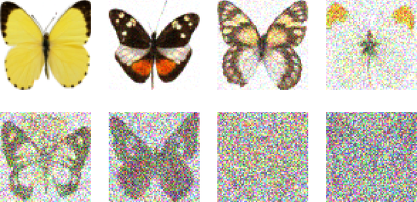
If you compare the results from our scheduler with those of DDPMScheduler, you may notice that they are not exactly the same, but they’re similar enough to explore training the model with our noise scheduler.

The Math

Let’s dive into the underlying math that explains how noise is added to the original images. One thing to remember is that there are many notations and approaches in the literature. For example, in some papers, the noise schedule is parametrized continuously, so t runs from 0 (no noise) to 1 (fully corrupted), as we did in our corrupt function. Other papers use a discrete time approach in which the timesteps are integers and run from 0 to a large number T, typically 1,000. It is possible to convert between these two approaches the way we did with our SimpleScheduler class—make sure you’re consistent when comparing different models. We’ll stick with the discrete time approach here.

A good place to start for going deeper into the math is the DDPM paper or the “Annotated Diffusion Model” blog post. If you feel this section is too dense, it’s OK to focus on the high-level concepts and come back to the math later on.

Let’s kick things off by defining how to do a single noise step to go from timestep t – 1 to timestep t. As mentioned earlier, the idea is to add Gaussian noise ($ϵ$). The noise has unit variance, which controls the spread of the noise values. By adding this noise to the previous step’s image, we gradually corrupt the original image, which is a key part of the diffusion model’s training process:

$${𝐱}_t={𝐱}_{t-1}+ϵ$$

To control the amount of noise added at each step, let’s introduce ${\beta }_t$. This parameter is defined for all timesteps t and specifies how much noise should be added at each step. In other words, ${𝐱}_t$ is a mix of ${𝐱}_{t-1}$ and some random noise scaled by ${\beta }_t$. This allows us to gradually increase the amount of noise added to the image as we move through the timesteps, which is a key part of the diffusion model’s training process:

$${𝐱}_t=\sqrt{1-{\beta }_t}{𝐱}_{t-1}+\sqrt{{\beta }_t}ϵ$$

We can further define the noise addition process as a distribution, where the noisy ${𝐱}_t$ has a mean $\sqrt{1-{\beta }_t}{𝐱}_{t-1}$ and a variance of ${\beta }_t$. This distribution helps us model the noise addition process more accurately. This is what the formula looks like in distribution form:

$$q\left({𝐱}_t\right|{𝐱}_{t-1})=𝒩({𝐱}_t;\sqrt{1-{\beta }_t}{𝐱}_{t-1},{\beta }_t𝐈)$$

We’ve now defined a distribution to sample $x$ conditioned on the previous value. To get the noisy input at timestep t, we could begin at t = 0 and repeatedly apply this single step, which would be very inefficient. Instead, we can find a formula to move to any timestep t in one go by doing the reparameterization trick. The idea is to precompute the noise schedule, which is defined by the ${\beta }_t$ values. We can then define ${\alpha }_t=1-{\beta }_t$ and $\overline{\alpha }$ as the cumulative product of all the $\alpha$ values up to time t, which can be expressed as ${\overline{\alpha }}_t:={\Pi }_{s=1}^t{\alpha }_s$. Using these tools and notation, we can redefine the distribution and how to sample at a particular time. The new distribution, $q\left({𝐱}_t\right|{𝐱}_{t-1})$, has a mean of ${\overline{\alpha }}_t{𝐱}_{t-1}$ and a variance of $(1-{\overline{\alpha }}_t)𝐈$:

$$q\left({𝐱}_t\right|{𝐱}_{t-1})=𝒩({𝐱}_t;{\overline{\alpha }}_t{𝐱}_{t-1},(1-{\overline{\alpha }}_t)𝐈)$$

Exploring this reparameterization trick is part of the challenges at the end of the chapter. We can now sample a noisy image at timestep t by using the following formula:

$$x_t=\sqrt{{\overline{\alpha }}_t}{x}_0+\sqrt{1-{\overline{\alpha }}_t}ϵ$$

The equation for $x_t$ shows that the noisy input at timestep t is a combination of the original image $x_0$ (scaled by $\sqrt{{\overline{\alpha }}_t}$) and $ϵ$ (scaled by $\sqrt{1-{\overline{\alpha }}_t}$). Note that we can now calculate a sample directly without looping over all previous timesteps, making it much more efficient for training diffusion models.

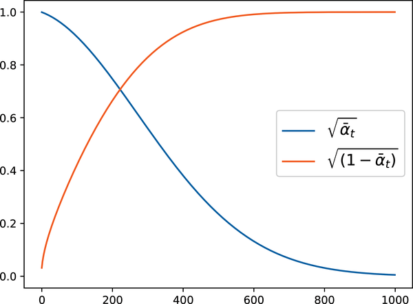
In the diffusers library, the $\overline{\alpha }$ values are stored in scheduler.alphas_cumprod. Knowing this, we can plot the scaling factors for the original image $x_0$ and the noise $ϵ$ across the different timesteps for a given scheduler. The diffusers library allows us to control the beta values by defining its initial value (beta_start), final value (beta_end), and how the values will step, for example, linearly (beta_schedule="linear"). The following plot for the DDPMScheduler describes the amount of noise (orange line) added to the input image (blue line). We can see that the noise is scaled up more as we have more timesteps, as expected:

from genaibook.core import plot_scheduler

plot_scheduler(
    DDPMScheduler(beta_start=0.001, beta_end=0.02, beta_schedule="linear")
)

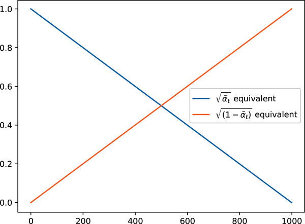
Our SimpleScheduler just linearly mixes between the original image and noise, as we can see if we plot the scaling factors (equivalent to $\sqrt{{\overline{\alpha }}_t}$ and $\sqrt{(1-{\overline{\alpha }}_t)}$ in the DDPM case):

plot_scheduler(SimpleScheduler())

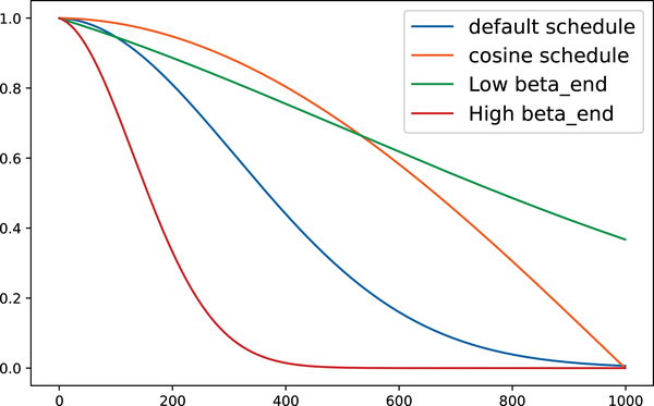
A good noise schedule will ensure the model sees a mix of images at different noise levels. The best choice will differ based on the training data. Visualizing a few more options, note the following:

• Setting beta_end too low means we never completely corrupt the image, so the model will never see anything like the random noise used as a starting point for inference.

• Setting beta_end extremely high means that most of the timesteps are spent on almost complete noise, resulting in poor training performance.

• Different beta schedules give different curves. The cosine schedule is popular, as it smoothly transitions from the original image to the noise.

Let’s visualize the comparison of different DDPMScheduler schedulers, varying hyperparameters and β schedules, with the following plot:

fig, (ax) = plt.subplots(1, 1, figsize=(8, 5))
plot_scheduler(
    DDPMScheduler(beta_schedule="linear"),
    label="default schedule",
    ax=ax,
    plot_both=False,
)
plot_scheduler(
    DDPMScheduler(beta_schedule="squaredcos_cap_v2"),
    label="cosine schedule",
    ax=ax,
    plot_both=False,
)
plot_scheduler(
    DDPMScheduler(beta_start=0.001, beta_end=0.003, beta_schedule="linear"),
    label="Low beta_end",
    ax=ax,
    plot_both=False,
)
plot_scheduler(
    DDPMScheduler(beta_start=0.001, beta_end=0.1, beta_schedule="linear"),
    label="High beta_end",
    ax=ax,
    plot_both=False,
)

Note

All the schedules shown here are called variance preserving (VP), meaning that the variance of the model input is kept close to 1 across the entire schedule. You may also encounter variance exploding (VE), formulations where noise is added to the original image in different amounts (resulting in high-variance inputs). Our SimpleScheduler is almost a VP schedule, but the variance is not quite preserved because of the linear interpolation.

The importance of exposing the model to a good mix of noised images—including pure noise, which is the initial state for inference—was explored in a paper titled “Common Diffusion Noise Schedules and Sample Steps Are Flawed”, which showed that some diffusion models were not able to generate images too bright or too dark because the training schedule didn’t cover all states. As with many diffusion-related topics, a constant stream of new papers is exploring the topic of noise schedules, so by the time you read this, there will likely be an extensive collection of options to try out.⁹

Effect of Input Resolution and Scaling

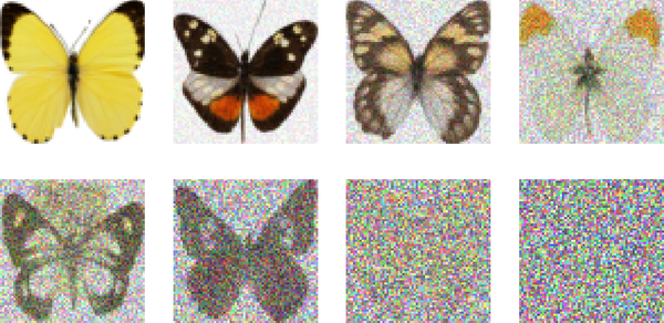
One aspect of noise schedules that has mostly been overlooked until recently is the effect of the input size and scaling. Many papers test potential schedulers on small-scale datasets and at low resolution and then use the best-performing scheduler to train their final models on larger images. The problem with this can be seen if we add the same amount of noise to two images of different sizes, as shown in Figure 4-6.

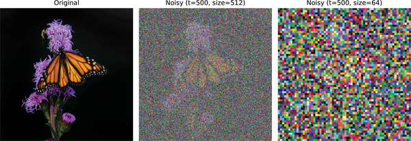
Figure 4-6. Applying the same amount of input noise to images with different resolutions

Images at high resolution tend to contain a lot of redundant information. This means that even if a single pixel is obscured by noise, the surrounding pixels have enough information to reconstruct the original image. This is different for low-resolution images, where a single pixel can contain a lot of useful information. Adding the same amount of noise to a low-resolution image will result in a much more corrupted image than adding the equivalent amount of noise to a high-resolution image.

Two independent papers from early 2023 thoroughly investigated this effect. Each used the new insights to train models capable of generating high-resolution outputs without requiring any of the tricks that have previously been necessary. Simple diffusion introduced a method for adjusting the noise schedule based on the input size, allowing a schedule optimized on low-resolution images to be appropriately modified for a new target resolution. The other paper performed similar experiments and noted another critical variable: input scaling. That is, how do we represent our images? If the images are represented as floats between 0 and 1, they will have a lower variance than the noise (typically unit variance). Thus, the signal-to-noise ratio will be lower for a given noise level than if the images were represented as floats between –1 and 1 (which we used in the preceding training example) or something else. Scaling the input images shifts the signal-to-noise ratio, so modifying this scaling is another way to adjust when training on larger images. This paper, in fact, recommends input scaling as an easy way to adapt training for different image sizes. It is also possible to adjust the noise schedule depending on the resolution, but then it’s more difficult to find the optimal schedule because several hyperparameters are involved. Here we see the effect of input scaling:

import numpy as np
from genaibook.core import load_image, SampleURL

scheduler = DDPMScheduler(beta_end=0.05, beta_schedule="scaled_linear")
image = load_image(
    SampleURL.DogExample,
    size=((512, 512)),
    return_tensor=True,
)

t = torch.tensor(300)  # The timestep we're noising to
scales = np.linspace(0.1, 1.0, 4)

images = [image]
noise = torch.randn_like(image)
for b in reversed(scales):
    noised = (
        scheduler.add_noise(b * (image * 2 - 1), noise, t).clip(-1, 1) * 0.5
        + 0.5
    )
    images.append(noised)

show_images(
    images[1:],
    nrows=1,
    titles=[f"Scale: {b}" for b in reversed(scales)],
    figsize=(15, 5),
)

All the images have the same input noise applied, corresponding to step t=300, but we multiply the input image by different scale factors. The noise is more noticeable as the scale affects the image more. The scale also decreases the dynamic range (or variance), resulting in darker-looking inputs.¹⁰

In Depth: UNets and Alternatives

Let’s address the actual model that makes the all-important predictions. To recap, this model must be capable of taking in a noisy image and outputting its noise, hence enabling denoising the input image. This requires a model that can take in an image of arbitrary size and output an image of the same size. Furthermore, the model should be able to make precise predictions at the pixel level while capturing higher-level information about the image. A popular approach is to use an architecture called a UNet. UNets were invented in 2015 for medical image segmentation and have since become a popular choice for various image-related tasks.

Like the AutoEncoders and VAEs we looked at in the previous chapter, UNets are made up of a series of downsampling and upsampling blocks. The downsampling blocks are responsible for reducing the image size, while the upsampling blocks are responsible for increasing the image size. The downsampling blocks typically comprise a series of convolutional layers, followed by a pooling or downsampling layer.¹¹ The upsampling blocks generally include a series of convolutional layers, followed by an upsampling or transposed convolution layer. The transposed convolution layer is a particular type of convolutional layer that increases the size of the image rather than reducing it.

Regular AutoEncoders and VAE are not good choices for this task because they are less capable of making precise predictions at the pixel level since they must reconstruct the images from the low-dimensional latent space. In a UNet, the downsampling and upsampling blocks are connected by skip connections, which allow information to flow directly from the downsampling blocks to the upsampling blocks. This allows the model to make precise predictions at the pixel level while also capturing higher-level information about the image as a whole.

A Simple UNet

To better understand the structure of a UNet, let’s build a simple one from scratch. Figure 4-7 shows the architecture diagram of a basic UNET.

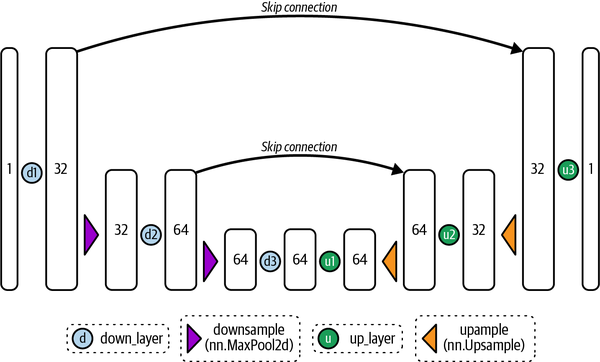
Figure 4-7. Architecture of a basic UNet

We’ll design a UNet that works with single-channel images (e.g., grayscale images), which we could use to build a diffusion model for datasets such as MNIST. We’ll use three layers in the downsampling path and another three in the upsampling path. Each layer consists of a convolution followed by an activation function and an upsampling or downsampling step, depending on whether they are in the encoding or decoding path. The skip connections, as mentioned, directly connect the downsampling blocks to the upsampling ones. There are multiple ways to implement the skip connections.

One approach, which we’ll use here, is to add the output of the downsampling block to the input of the corresponding upsampling block. Another method is concatenating the downsampling block’s output to the upsampling block’s input. We could even add some additional layers in the skip connections.

Let’s keep things simple for now with the initial approach. Here’s what this network looks like in code:

from torch import nn


class BasicUNet(nn.Module):
    """A minimal UNet implementation."""

    def __init__(self, in_channels=1, out_channels=1):
        super().__init__()
        self.down_layers = nn.ModuleList(
            [
                nn.Conv2d(in_channels, 32, kernel_size=5, padding=2),
                nn.Conv2d(32, 64, kernel_size=5, padding=2),
                nn.Conv2d(64, 64, kernel_size=5, padding=2),
            ]
        )
        self.up_layers = nn.ModuleList(
            [
                nn.Conv2d(64, 64, kernel_size=5, padding=2),
                nn.Conv2d(64, 32, kernel_size=5, padding=2),
                nn.Conv2d(32, out_channels, kernel_size=5, padding=2),
            ]
        )

        # Use the SiLU activation function, which has been shown to work well
        # due to different properties (smoothness, non-monotonicity, etc.).
        self.act = nn.SiLU()
        self.downscale = nn.MaxPool2d(2)
        self.upscale = nn.Upsample(scale_factor=2)

    def forward(self, x):
        h = []
        for i, l in enumerate(self.down_layers):
            x = self.act(l(x))
            if i < 2:  # For all but the third (final) down layer:
                h.append(x)  # Storing output for skip connection
                x = self.downscale(x)  # Downscale ready for the next layer

        for i, l in enumerate(self.up_layers):
            if i > 0:  # For all except the first up layer
                x = self.upscale(x)  # Upscale
                x += h.pop()  # Fetching stored output (skip connection)
            x = self.act(l(x))

        return x

If you take a grayscale input image of shape (1, 28, 28), the path through the model would be as follows:

1. The image goes through the downscaling block. The first layer, a 2D convolution with 32 filters, will make it of shape [32, 28, 28].

2. The image is then downscaled with max pooling, making it of shape [32, 14, 14]. The MNIST dataset contains white numbers drawn on a black background (where black is represented by the number zero). We choose max pooling to select the largest values in a region and thus focus on the brightest pixels.¹²

3. The image goes through the second downscaling block. The second layer, a 2D convolution with 64 filters, will make it of shape [64, 14, 14].

4. After another downscaling, the shape is [64, 7, 7].

5. There is a third layer in the downscaling block, but no downscaling this time because we are already using very small 7 × 7 blocks. This will keep the shape of [64, 7, 7].

6. We do the same process but in inverse, upscaling to [64, 14, 14], [32, 14, 14], and finally [1, 28, 28].

A diffusion model trained with this architecture on MNIST produces the samples shown in Figure 4-8 (code included in the supplementary material but omitted here for brevity).

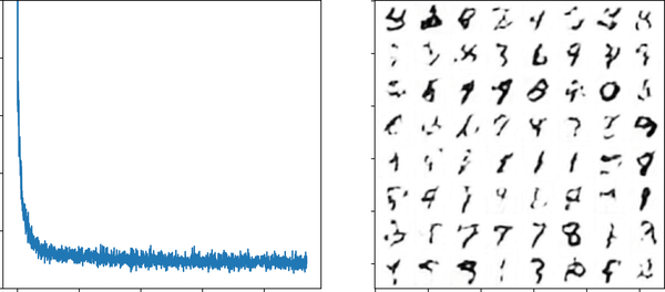
Figure 4-8. Loss and generations of a basic UNet

Improving the UNet

This simple UNet works for this relatively easy task. How can we handle more-complex data? Here are some options:

Add more parameters

This can be accomplished by using multiple convolutional layers in each block, using a larger number of filters in each convolutional layer, or making the network deeper.

Add normalization, such as batch normalization

Batch normalization can help the model learn more quickly and reliably by ensuring that the outputs of each layer are centered around 0 and have a standard deviation of 1.

Add regularization, such as dropout

Dropout helps prevent overfitting to the training data, which is essential when working with smaller datasets.

Add attention

Introducing self-attention layers allows the model to focus on different parts of the image at different times, which can help the UNet learn more-complex functions. Adding transformer-like attention layers also lets us increase the number of learnable parameters. The downside is that attention layers are much more expensive to compute than regular convolutional layers at higher resolutions, so we typically use them only at lower resolutions (e.g., the lower-resolution blocks in the UNet).

For comparison, Figure 4-9 shows the results on MNIST when using the UNet implementation in the diffusers library, which features the aforementioned improvements.

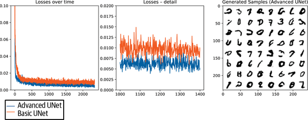
Figure 4-9. Loss and generations from the diffusers UNet, with several improvements over the basic architecture

Alternative Architectures

More recently, several alternative architectures have been proposed for diffusion models (Figure 4-10).

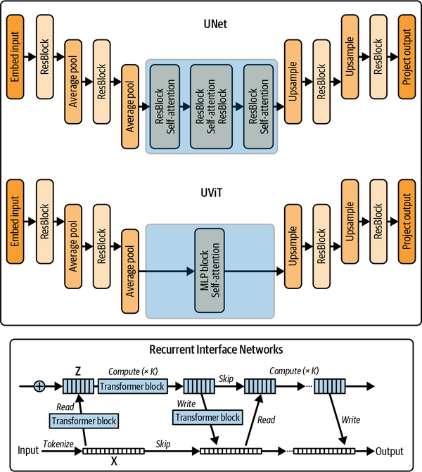
Figure 4-10. Comparison of UNet with UViT and RIN

These architectures include the following:

Transformers

The Diffusion Transformers paper showed that a transformer-based architecture can train a diffusion model with excellent results. However, the compute and memory requirements of the transformer architecture remain a challenge for very high resolutions.

UViT

The UViT architecture from the Simple Diffusion paper aims to get the best of both worlds by replacing the middle layers of the UNet with a large stack of transformer blocks. A key insight of this paper is that focusing most of the compute at the lower-resolution blocks of the UNet allows for more efficient training of high-resolution diffusion models. For very high resolutions, they do some additional preprocessing using something called a wavelet transform to reduce the spatial resolution of the input image while keeping as much information as possible through additional channels, again reducing the amount of compute spent on the higher spatial resolutions.

Recurrent Interface Networks (RINs)

The RIN paper takes a similar approach, first mapping the high-resolution inputs to a more manageable and lower-dimensional latent representation, which is then processed by a stack of transformer blocks before being decoded back out to an image. Additionally, the RIN paper introduces the idea of recurrence, where information is passed to the model from the previous processing step. This can benefit the iterative improvement that diffusion models are designed to perform.

Some high-quality diffusion transformer models include Flux, Stable Diffusion 3, PixArt-Σ, and the text-to-video Sora. It remains to be seen whether transformer-based approaches completely supplant UNets as the go-to architecture for diffusion models or whether hybrid approaches like the UViT and RIN architectures will be the most effective.

In Depth: Diffusion Objectives

We’ve discussed diffusion models taking a noisy input and learning to denoise it. At first glance, you might assume that the network’s natural prediction target is the image’s denoised version, which we’ll call x0. However, we compared the model prediction in the code with the unit-variance noise used to create the noisy version (often called the epsilon objective, eps). The two appear mathematically identical since if we know the noise and the timestep, we can derive x0, and vice versa. While this is true, the objective choice has some subtle effects on how large the loss is at different timesteps and, thus, which noise levels the model learns best to denoise. Predicting noise is easier for the model than directly predicting the target data. This is because the noise follows a known distribution at each step, and predicting the difference between two steps is often simpler than predicting the absolute values of the target data.

To gain some intuition, let’s visualize some different objectives across different timesteps. The input image and the random noise in Figure 4-11 are the same (first two rows in the illustration), but the noised images in the third row have different amounts of added noise depending on the timestep.

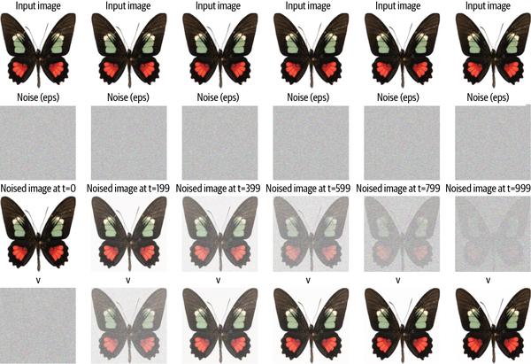
Figure 4-11. Comparing eps versus x0 versus v objectives: eps tries to predict the noise added at each timestep, x0 predicts the denoised image, and v uses a mixture of the two

At extremely low noise levels, the x0 objective is trivially easy (the noised image is almost the same as the input), while predicting the noise accurately is almost impossible. Likewise, at extremely high noise levels, the eps objective is straightforward (the noised image is almost equal to the pure noise added), while predicting the denoised image accurately is almost impossible. If we use the x0 objective, our training will put less weight on lower noise levels.

Neither case is ideal, and so additional objectives have been introduced that have the model predict a mix of x0 and eps at different timesteps. The velocity (v) objective, shown in the last row of the illustration, is one such objective, which is defined as $v=\sqrt{\overline{\alpha }}·ϵ+\sqrt{1-\overline{\alpha }}·x_0$. The eps objective remains one of the most preferred approaches, but it’s important to be aware of its disadvantages and the existence of other objectives.

Note

A group of researchers at NVIDIA worked to unify the different formulations of diffusion models into a consistent framework with a clear separation of design choices. This allowed them to identify changes in the sampling and training processes, resulting in better performance, leading to what is known as k-diffusion. If you’re interested in learning more about the different objectives, scalings, and nuances of the diffusion model formulations, we recommend reading the EDM paper for a more in-depth discussion.

Project Time: Train Your Diffusion Model

OK, that’s enough theory. It’s now time for you to train your unconditional diffusion model. As before, you’ll train a model to generate new images. The main challenge of this project will be creating or finding a good dataset you can use for this.

In case you want to use an existing dataset, a good starting point is to filter for image-classification datasets on the Hugging Face Hub and pick one of your liking. One of the main questions you will want to answer is which part of the dataset you want to use for training. Will you use the whole dataset, as before, so that the model generates digits? Or will you use a specific class (e.g., cats, so that we get a cats expert model)? Or will you use a subset of the dataset (e.g., only images with a certain resolution)?

If you want to upload a new dataset instead, the first step will be to find and access the data. To share a dataset, the most straightforward approach is to use the ImageFolder feature of the datasets library. You can then upload the dataset to the Hugging Face Hub and use it in your project.

Once you have the data, think about the preprocessing steps, the model definition, and the training loop. You can use the code from the chapter as a starting point and modify it to fit your dataset.

Summary

We started the chapter using high-level pipelines to run inference of diffusion models. We ended up training our diffusion model from scratch and diving into each component. Let’s do a brief recap.

The goal is to train a model, usually a UNet, that receives noisy images as input and can predict the noise part of that image. When training our model, we add noise in different magnitudes according to a random number of timesteps. One of the challenges we saw was that to add noise at a high number of steps, 900, for example, we would need to do a high number of noise iterations. To fix this, we use the reparameterization trick, which allows us to obtain the noisy input at a specific timestep directly. The model is trained to minimize the difference between the noise predictions and the actual input noise. For inference, we do an iterative refinement process in which the model refines the initial random input. Rather than keeping the final prediction of a single diffusion step, we iteratively modify the input x by a small amount in the direction of that prediction. This, of course, is one of the reasons doing inference with diffusion models tends to be slow and becomes one of its main disadvantages compared to models like GANs.

The diffusion world is fast-moving, so many advances exist (e.g., the scheduler, the model, the training techniques, and so on). This chapter focused on foundations that will allow us to jump to conditional generation (e.g., generating an image conditioned on an input prompt) and provide a background for you to dive deeper into the diffusion world. Some of the readings through this chapter can help you dive deeper.

For additional readings, we suggest reviewing the following:

• The “Annotated Diffusion Model” blog post, which does a technical write-up of the DDPM paper

• Lilian Weng’s write-up, which is excellent for a deeper dive into the math

• The “Denoising Diffusion Probabilistic Models” paper itself

• Karras’s work on unifying the formulations of diffusion models

• “Simple Diffusion: End-to-End Diffusion for High Resolution Images”, which explains how to adjust the sample schedule for different sizes

Exercises

1. Explain the diffusion inference algorithm.

2. What’s the role of the noise scheduler?

3. When creating a training dataset of images, which characteristics are important to watch?

4. Why do we randomly flip training images?

5. How can we evaluate the generations of diffusion models?

6. How do the values of beta_end impact the diffusion process?

7. Why do we use UNets rather than VAEs as the main model for diffusion?

8. What benefits and challenges are faced when incorporating techniques from transformers (like attention layers or a transformer-based architecture) to diffusion?

You can find the solutions to these exercises and the following challenges in the book’s GitHub repository.

Challenges

1. Reparameterization trick. Show that

   $${𝐱}_t=\sqrt{1-{\beta }_t}{𝐱}_{t-1}+\sqrt{{\beta }_t}ϵ$$

   is equivalent to

   $${𝐱}_t=\sqrt{{\overline{\alpha }}_t}{𝐱}_0+\sqrt{1-{\overline{\alpha }}_t}ϵ$$

   Note that this is not a trivial example and is not required to use diffusion models. We recommend reviewing “A Beginner’s Guide to Diffusion Models: Understanding the Basics and Beyond” for guidance. An important thing to know is how to merge two Gaussians: if you have two Gaussians with different variance, $𝒩({\mu }_1,{\sigma }_1^2)$ and $𝒩({\mu }_2,{\sigma }_2^2)$, the resulting Gaussian is $𝒩({\mu }_1+{\mu }_2,{\sigma }_1^2+{\sigma }_2^2)$.

2. DDIM scheduler. This chapter uses the DDPM scheduler, sometimes requiring hundreds or thousands of steps to achieve high-quality results. Recent research has explored achieving good generations with as few steps as possible, down to even one or two. The diffusers library contains multiple schedulers such as the DDIMScheduler from the “Denoising Diffusion Implicit Models” paper. Create some images using the DDIMScheduler. This chapter’s sampling section required 1,000 steps with the DDPMScheduler. How many steps are required for you to generate images with similar quality? Experiment switching the scheduler for google/ddpm-celebahq-256 and compare both schedulers.

References

1. Bansal, Arpit, et al. “Cold Diffusion: Inverting Arbitrary Image Transforms Without Noise.” arXiv, August 19, 2022. http://arxiv.org/abs/2208.09392.

2. Chen, Ting. “On the Importance of Noise Scheduling for Diffusion Models.” arXiv, May 21, 2023. http://arxiv.org/abs/2301.10972.

3. Ho, Jonathan, et al. “Denoising Diffusion Probabilistic Models.” arXiv, December 16, 2020. http://arxiv.org/abs/2006.11239.

4. Hoogeboom, Emiel, et al. “Simple Diffusion: End-to-End Diffusion for High Resolution Images.” arXiv, December 12, 2023. http://arxiv.org/abs/2301.11093.

5. Jabri, Allan, et al. “Scalable Adaptive Computation for Iterative Generation.” arXiv, June 13 2023. http://arxiv.org/abs/2212.11972.

6. Karras, Tero, et al. “Elucidating the Design Space of Diffusion-Based Generative Models.” arXiv, October 11, 2022. http://arxiv.org/abs/2206.00364.

7. Lee, Tony, et al. “Holistic Evaluation of Text-to-Image Models.” arXiv, November 7, 2023. https://arxiv.org/abs/2311.04287.

8. Lin, Shanchuan, et al. “Common Diffusion Noise Schedules and Sample Steps Are Flawed.” arXiv, January 23, 2024. https://arxiv.org/abs/2305.08891.

9. Peebles, William, and Saining Xie. “Scalable Diffusion Models with Transformers.” arXiv, March 2, 2023. http://arxiv.org/abs/2212.09748.

10. Rogge, Niels, and Kashif Rasul. “The Annotated Diffusion Model.” Hugging Face blog, June 7, 2022. https://oreil.ly/mFHxe.

11. Ronneberger, Olaf, et al. “U-Net: Convolutional Networks for Biomedical Image Segmentation.” arXiv, May 18, 2015. http://arxiv.org/abs/1505.04597.

12. Song, Jiaming, et al. “Denoising Diffusion Implicit Models.” arXiv, October 5, 2022. https://arxiv.org/abs/2010.02502.

¹ There’s a lot of research about reducing the number of diffusion steps in inference; please check Challenge 2 in “Challenges” for an initial glimpse into the area.

² This is a subset of a dataset compiled by Ceyda Cinarel with butterflies extracted from the Smithsonian Institute.

³ torchvision is a PyTorch library that provides a wide range of tools for working with images. In the book, we’ll use this library only for data preprocessing transformations.

⁴ We used images larger than 64 × 64 to print beautiful butterflies in the book instead of pixelated ones.

⁵ The images were generated by the model we trained at a resolution of 64 × 64 and upscaled, so they’ll look pixelated.

⁶ ImageNet is one of the most popular Computer Vision benchmarks. It contains millions of images in thousands of categories, making it a popular dataset for training and benchmarking base models.

⁷ For a practical deep dive into evaluating diffusion models, we suggest reviewing the diffusers library’s “Evaluating Diffusion Models” documentation.

⁸ The Gaussian noise is added with torch.rand_like().

⁹ The diffusers documentation page on schedulers can be a good place to get started with the multiple schedulers variants.

¹⁰ In this regime, input images are normalized before being passed to the model to not reduce variance so drastically.

¹¹ Pooling is the method to choose the information to preserve when downsampling the output from a previous layer. Common strategies include average pooling, which reduces a patch to its average value, or max pooling, which selects the maximum value in a given patch. Pooling is applied independently to all the channels of the input tensor.

¹² For visualization purposes, we show MNIST as black numbers on a white background, but the training dataset uses the opposite.