Generative Deep Learning

Chapter 4. Generative Adversarial Networks

On Monday, December 5, 2016, at 2:30 p.m., Ian Goodfellow of Google Brain presented a tutorial entitled “Generative Adversarial Networks” to the delegates of the Neural Information Processing Systems (NIPS) conference in Barcelona.¹ The ideas presented in the tutorial are now regarded as one of the key turning points for generative modeling and have spawned a wide variety of variations on his core idea that have pushed the field to even greater heights.

This chapter will first lay out the theoretical underpinning of generative adversarial networks (GANs). You will then learn how to use the Python library Keras to start building your own GANs.

First though, we shall take a trip into the wilderness to meet Gene…

Ganimals

One afternoon, while walking through the local jungle, Gene sees a woman thumbing through a set of black and white photographs, looking worried. He goes over to ask if he can help.

The woman introduces herself as Di, a keen explorer, and explains that she is hunting for the elusive ganimal, a mythical creature that is said to roam around the jungle. Since the creature is nocturnal, she only has a collection of nighttime photos of the beast that she once found lying on the floor of the jungle, dropped by another ganimal enthusiast. Some of these photos are shown in Figure 4-1. Di makes money by selling the images to collectors but is starting to worry, as she hasn’t actually ever seen the creatures and is concerned that her business will falter if she can’t produce more original photographs soon.

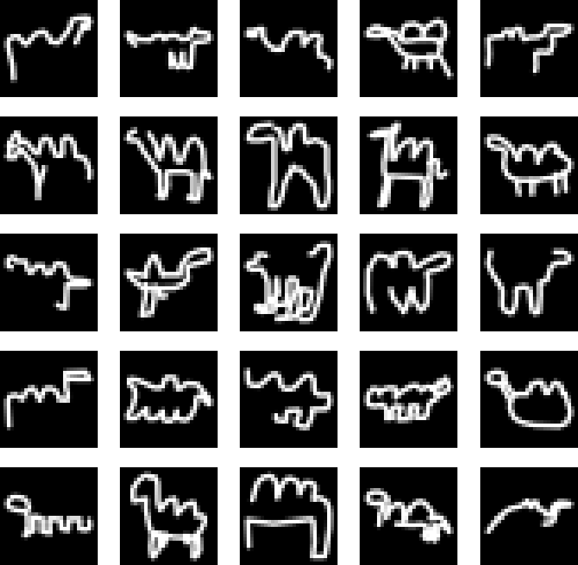
Figure 4-1. Original ganimal photographs

Being a keen photographer, Gene decides to help Di. He agrees to search for the ganimal himself and give her any photographs of the nocturnal beast that he manages to take.

However, there is a problem. Since Gene has never seen a ganimal, he doesn’t know how to produce good photos of the creature, and also, since Di has only ever sold the photos she found, she cannot even tell the difference between a good photo of a ganimal and a photo of nothing at all.

Starting from this state of ignorance, how can they work together to ensure Gene is eventually able to produce impressive ganimal photographs?

They come up with following process. Each night, Gene takes 64 photographs, each in a different location with different random moonlight readings, and mixes them with 64 ganimal photos from the original collection. Di then looks at this set of photos and tries to guess which were taken by Gene and which are originals. Based on her mistakes, she updates her own understanding of how to discriminate between Gene’s attempts and the original photos. Afterwards, Gene takes another 64 photos and shows them to Di. Di gives each photo a score between 0 and 1, indicating how realistic she thinks each photo is. Based on this feedback, Gene updates the settings on his camera to ensure that next time, he takes photos that Di is more likely to rate highly.

This process continues for many days. Initially, Gene doesn’t get any useful feedback from Di, since she is randomly guessing which photos are genuine. However, after a few weeks of her training ritual, she gradually gets better at this, which means that she can provide better feedback to Gene so that he can adjust his camera accordingly in his training session. This makes Di’s task harder, since now Gene’s photos aren’t quite as easy to distinguish from the real photos, so she must again learn how to improve. This back-and-forth process continues, over many days and weeks.

Over time, Gene gets better and better at producing ganimal photos, until eventually, Di is once again resigned to the fact that she cannot tell the difference between Gene’s photos and the originals. They take Gene’s generated photos to the auction and the experts cannot believe the quality of the new sightings—they are just as convincing as the originals. Some examples of Gene’s work are shown in Figure 4-2.

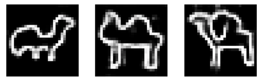
Figure 4-2. Samples of Gene’s ganimal photography

Introduction to GANs

The adventures of Gene and Di hunting elusive nocturnal ganimals are a metaphor for one of the most important deep learning advancements of recent years: generative adversarial networks.

Simply put, a GAN is a battle between two adversaries, the generator and the discriminator. The generator tries to convert random noise into observations that look as if they have been sampled from the original dataset and the discriminator tries to predict whether an observation comes from the original dataset or is one of the generator’s forgeries. Examples of the inputs and outputs to the two networks are shown in Figure 4-3.

Figure 4-3. Inputs and outputs of the two networks in a GAN

At the start of the process, the generator outputs noisy images and the discriminator predicts randomly. The key to GANs lies in how we alternate the training of the two networks, so that as the generator becomes more adept at fooling the discriminator, the discriminator must adapt in order to maintain its ability to correctly identify which observations are fake. This drives the generator to find new ways to fool the discriminator, and so the cycle continues.

To see this in action, let’s start building our first GAN in Keras, to generate pictures of nocturnal ganimals.

Your First GAN

First, you’ll need to download the training data. We’ll be using the Quick, Draw! dataset from Google. This is a crowdsourced collection of 28 × 28–pixel grayscale doodles, labeled by subject. The dataset was collected as part of an online game that challenged players to draw a picture of an object or concept, while a neural network tries to guess the subject of the doodle. It’s a really useful and fun dataset for learning the fundamentals of deep learning. For this task you’ll need to download the camel numpy file and save it into the ./data/camel/ folder in the book repository.² The original data is scaled in the range [0, 255] to denote the pixel intensity. For this GAN we rescale the data to the range [–1, 1].

Running the notebook 04_01_gan_camel_train.ipynb in the book repository will start training the GAN. As in the previous chapter on VAEs, you can instantiate a GAN object in the notebook, as shown in Example 4-1, and play around with the parameters to see how it affects the model.

Example 4-1. Defining the GAN

gan = GAN(input_dim = (28,28,1)
            , discriminator_conv_filters = [64,64,128,128]
            , discriminator_conv_kernel_size = [5,5,5,5]
            , discriminator_conv_strides = [2,2,2,1]
            , discriminator_batch_norm_momentum = None
            , discriminator_activation = 'relu'
            , discriminator_dropout_rate = 0.4
            , discriminator_learning_rate = 0.0008
            , generator_initial_dense_layer_size = (7, 7, 64)
            , generator_upsample = [2,2, 1, 1]
            , generator_conv_filters = [128,64, 64,1]
            , generator_conv_kernel_size = [5,5,5,5]
            , generator_conv_strides = [1,1, 1, 1]
            , generator_batch_norm_momentum = 0.9
            , generator_activation = 'relu'
            , generator_dropout_rate = None
            , generator_learning_rate = 0.0004
            , optimiser = 'rmsprop'
            , z_dim = 100
            )

Let’s first take a look at how we build the discriminator.

The Discriminator

The goal of the discriminator is to predict if an image is real or fake. This is a supervised image classification problem, so we can use the same network architecture as in Chapter 2: stacked convolutional layers, followed by a dense output layer.

In the original GAN paper, dense layers were used in place of the convolutional layers. However, since then, it has been shown that convolutional layers give greater predictive power to the discriminator. You may see this type of GAN called a DCGAN (deep convolutional generative adversarial network) in the literature, but now essentially all GAN architectures contain convolutional layers, so the “DC” is implied when we talk about GANs. It is also common to see batch normalization layers in the discriminator for vanilla GANs, though we choose not to use them here for simplicity.

The full architecture of the discriminator we will be building is shown in Figure 4-4.

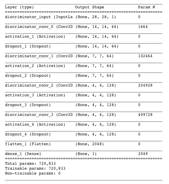
Figure 4-4. The discriminator of the GAN

The Keras code to build the discriminator is provided in Example 4-2.

Example 4-2. The discriminator

discriminator_input = Input(shape=self.input_dim, name='discriminator_input') 
x = discriminator_input

for i in range(self.n_layers_discriminator): 

    x = Conv2D(
        filters = self.discriminator_conv_filters[i]
        , kernel_size = self.discriminator_conv_kernel_size[i]
        , strides = self.discriminator_conv_strides[i]
        , padding = 'same'
        , name = 'discriminator_conv_' + str(i)
        )(x)

    if self.discriminator_batch_norm_momentum and i > 0:
        x = BatchNormalization(momentum = self.discriminator_batch_norm_momentum)(x)

    x = Activation(self.discriminator_activation)(x)

    if self.discriminator_dropout_rate:
        x = Dropout(rate = self.discriminator_dropout_rate)(x)

x = Flatten()(x) 
discriminator_output= Dense(1, activation='sigmoid'
    , kernel_initializer = self.weight_init)(x) 

discriminator = Model(discriminator_input, discriminator_output) 

Define the input to the discriminator (the image).

Stack convolutional layers on top of each other.

Flatten the last convolutional layer to a vector.

Dense layer of one unit, with a sigmoid activation function that transforms the output from the dense layer to the range [0, 1].

The Keras model that defines the discriminator—a model that takes an input image and outputs a single number between 0 and 1.

Notice how we use a stride of 2 in some of the convolutional layers to reduce the size of the tensor as it passes through the network, but increase the number of channels (1 in the grayscale input image, then 64, then 128).

The sigmoid activation in the final layer ensures that the output is scaled between 0 and 1. This will be the predicted probability that the image is real.

The Generator

Now let’s build the generator. The input to the generator is a vector, usually drawn from a multivariate standard normal distribution. The output is an image of the same size as an image in the original training data.

This description may remind you of the decoder in a variational autoencoder. In fact, the generator of a GAN fulfills exactly the same purpose as the decoder of a VAE: converting a vector in the latent space to an image. The concept of mapping from a latent space back to the original domain is very common in generative modeling as it gives us the ability to manipulate vectors in the latent space to change high-level features of images in the original domain.

The architecture of the generator we will be building is shown in Figure 4-5.

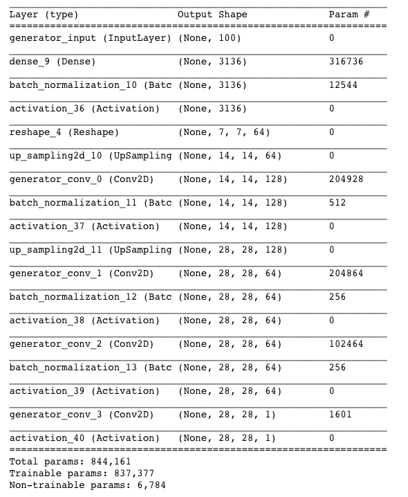
Figure 4-5. The generator

First though, we need to introduce a new layer type: the upsampling layer.

Upsampling

In the decoder of the variational autoencoder that we built in the previous chapter, we doubled the width and height of the tensor at each layer using Conv2DTranspose layers with stride 2. This inserted zero values in between pixels before performing the convolution operations.

In this GAN, we instead use the Keras Upsampling2D layer to double the width and height of the input tensor. This simply repeats each row and column of its input in order to double the size. We then follow this with a normal convolutional layer with stride 1 to perform the convolution operation. It is a similar idea to convolutional transpose, but instead of filling the gaps between pixels with zeros, upsampling just repeats the existing pixel values.

Both of these methods—Upsampling + Conv2D and Conv2DTranspose—are acceptable ways to transform back to the original image domain. It really is a case of testing both methods in your own problem setting and seeing which produces better results. It has been shown that the Conv2DTranspose method can lead to artifacts, or small checkerboard patterns in the output image (see Figure 4-6) that spoil the quality of the output. However, they are still used in many of the most impressive GANs in the literature and have proven to be a powerful tool in the deep learning practitioner’s toolbox—again, I suggest you experiment with both methods and see which works best for you.

Figure 4-6. Artifacts when using convolutional transpose layers³

The code for building the generator is given in Example 4-3.

Example 4-3. The generator

generator_input = Input(shape=(self.z_dim,), name='generator_input') 
x = generator_input

x = Dense(np.prod(self.generator_initial_dense_layer_size))(x) 

if self.generator_batch_norm_momentum:
    x = BatchNormalization(momentum = self.generator_batch_norm_momentum)(x)
x = Activation(self.generator_activation)(x)

x = Reshape(self.generator_initial_dense_layer_size)(x) 

if self.generator_dropout_rate:
    x = Dropout(rate = self.generator_dropout_rate)(x)

for i in range(self.n_layers_generator): 

    x = UpSampling2D()(x)
    x = Conv2D(
        filters = self.generator_conv_filters[i]
        , kernel_size = self.generator_conv_kernel_size[i]
        , padding = 'same'
        , name = 'generator_conv_' + str(i)
        )(x)

    if i < n_layers_generator - 1: 
        if self.generator_batch_norm_momentum:
            x = BatchNormalization(momentum = self.generator_batch_norm_momentum))(x)
        x = Activation('relu')(x)
    else:
        x = Activation('tanh')(x)


generator_output = x
generator = Model(generator_input, generator_output) 

Define the input to the generator—a vector of length 100.

We follow this with a Dense layer consisting of 3,136 units…

…which, after applying batch normalization and a ReLU activation function, is reshaped to a 7 × 7 × 64 tensor.

We pass this through four Conv2D layers, the first two preceded by Upsampling2D layers, to reshape the tensor to 14 × 14, then 28 × 28 (the original image size). In all but the last layer, we use batch normalization and ReLU activation (LeakyReLU could also be used).

After the final Conv2D layer, we use a tanh activation to transform the output to the range [–1, 1], to match the original image domain.

The Keras model that defines the generator—a model that accepts a vector of length 100 and outputs a tensor of shape [28, 28, 1].

Training the GAN

As we have seen, the architecture of the generator and discriminator in a GAN is very simple and not so different from the models that we looked at earlier. The key to understanding GANs is in understanding the training process.

We can train the discriminator by creating a training set where some of the images are randomly selected real observations from the training set and some are outputs from the generator. The response would be 1 for the true images and 0 for the generated images. If we treat this as a supervised learning problem, we can train the discriminator to learn how to tell the difference between the original and generated images, outputting values near 1 for the true images and values near 0 for the fake images.

Training the generator is more difficult as there is no training set that tells us the true image that a particular point in the latent space should be mapped to. Instead, we only want the image that is generated to fool the discriminator—that is, when the image is fed as input to the discriminator, we want the output to be close to 1.

Therefore, to train the generator, we must first connect it to the discriminator to create a Keras model that we can train. Specifically, we feed the output from the generator (a 28 × 28 × 1 image) into the discriminator so that the output from this combined model is the probability that the generated image is real, according to the discriminator. We can train this combined model by creating training batches consisting of randomly generated 100-dimensional latent vectors as input and a response which is set to 1, since we want to train the generator to produce images that the discriminator thinks are real.

The loss function is then just the binary cross-entropy loss between the output from the discriminator and the response vector of 1.

Crucially, we must freeze the weights of the discriminator while we are training the combined model, so that only the generator’s weights are updated. If we do not freeze the discriminator’s weights, the discriminator will adjust so that it is more likely to predict generated images as real, which is not the desired outcome. We want generated images to be predicted close to 1 (real) because the generator is strong, not because the discriminator is weak.

A diagram of the training process for the discriminator and generator is shown in Figure 4-7.

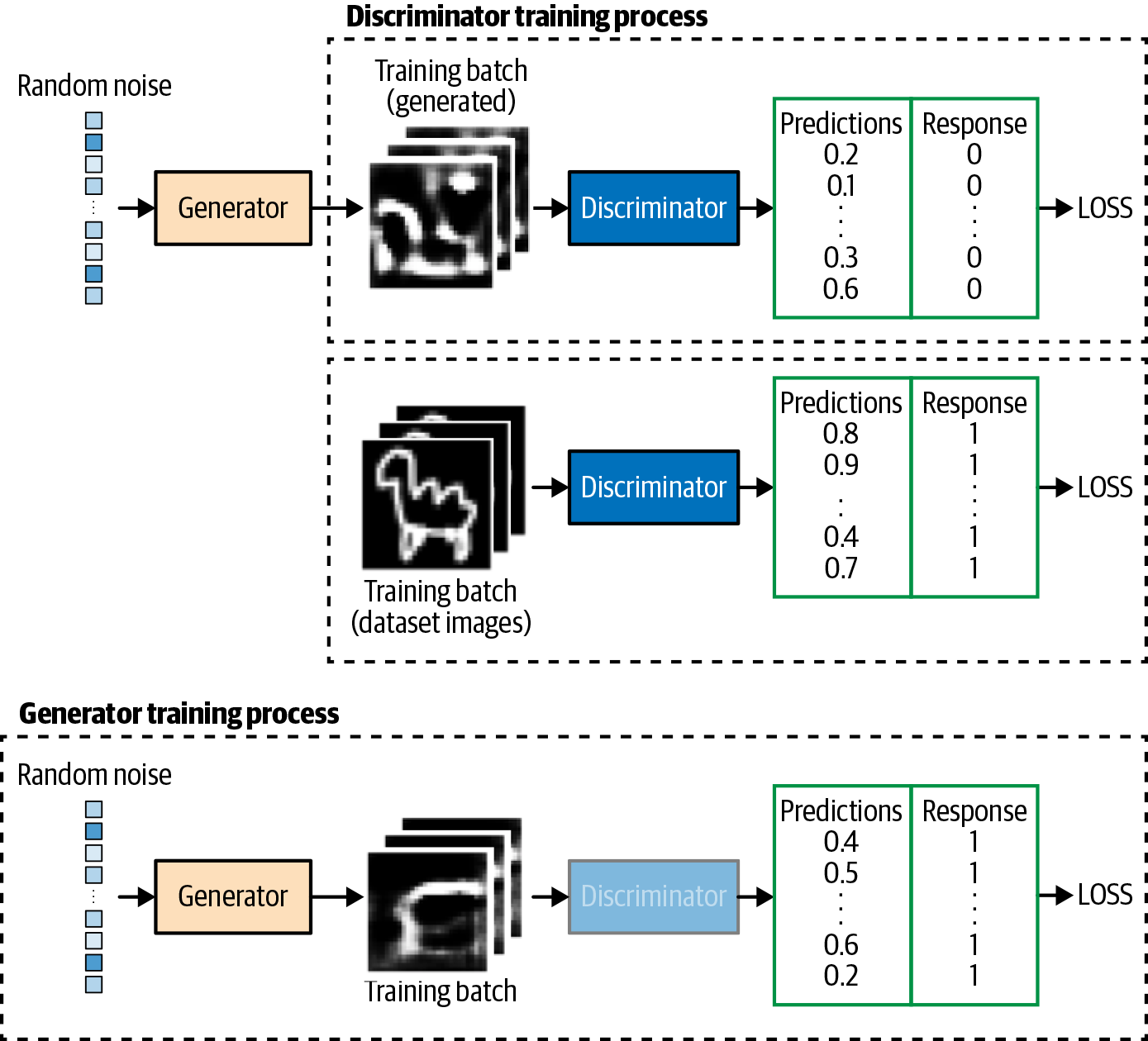
Figure 4-7. Training the GAN

Let’s see what this looks like in code. First we need to compile the discriminator model and the model that trains the generator (Example 4-4).

Example 4-4. Compiling the GAN

### COMPILE MODEL THAT TRAINS THE DISCRIMINATOR

self.discriminator.compile(
    optimizer= RMSprop(lr=0.0008)
    , loss = 'binary_crossentropy'
    ,  metrics = ['accuracy']
) 

### COMPILE MODEL THAT TRAINS THE GENERATOR

self.discriminator.trainable = False 
model_input = Input(shape=(self.z_dim,), name='model_input')
model_output = discriminator(self.generator(model_input))
self.model = Model(model_input, model_output) 

self.model.compile(
    optimizer=RMSprop(lr=0.0004)
    , loss='binary_crossentropy'
    , metrics=['accuracy']
) 

The discriminator is compiled with binary cross-entropy loss, as the response is binary and we have one output unit with sigmoid activation.

Next, we freeze the discriminator weights—this doesn’t affect the existing discriminator model that we have already compiled.

We define a new model whose input is a 100-dimensional latent vector; this is passed through the generator and frozen discriminator to produce the output probability.

Again, we use a binary cross-entropy loss for the combined model—the learning rate is slower than the discriminator as generally we would like the discriminator to be stronger than the generator. The learning rate is a parameter that should be tuned carefully for each GAN problem setting.

Then we train the GAN by alternating training of the discriminator and generator (Example 4-5).

Example 4-5. Training the GAN

def train_discriminator(x_train, batch_size):

    valid = np.ones((batch_size,1))
    fake = np.zeros((batch_size,1))

    # TRAIN ON REAL IMAGES
    idx = np.random.randint(0, x_train.shape[0], batch_size)
    true_imgs = x_train[idx]
    self.discriminator.train_on_batch(true_imgs, valid) 

    # TRAIN ON GENERATED IMAGES
    noise = np.random.normal(0, 1, (batch_size, z_dim))
    gen_imgs = generator.predict(noise)
    self.discriminator.train_on_batch(gen_imgs, fake) 


def train_generator(batch_size):

    valid = np.ones((batch_size,1))

    noise = np.random.normal(0, 1, (batch_size, z_dim))
    self.model.train_on_batch(noise, valid) 

epochs = 2000
batch_size = 64

for epoch in range(epochs):

    train_discriminator(x_train, batch_size)
    train_generator(batch_size)

One batch update of the discriminator involves first training on a batch of true images with the response 1…

…then on a batch of generated images with the response 0.

One batch update of the generator involves training on a batch of generated images with the response 1. As the discriminator is frozen, its weights will not be affected; instead, the generator weights will move in the direction that allows it to better generate images that are more likely to fool the discriminator (i.e., make the discriminator predict values close to 1).

After a suitable number of epochs, the discriminator and generator will have found an equilibrium that allows the generator to learn meaningful information from the discriminator and the quality of the images will start to improve (Figure 4-8).

Figure 4-8. Loss and accuracy of the discriminator and generator during training

By observing images produced by the generator at specific epochs during training (Figure 4-9), it is clear that the generator is becoming increasingly adept at producing images that could have been drawn from the training set.

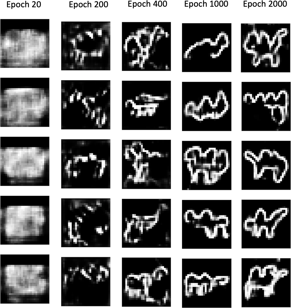
Figure 4-9. Output from the generator at specific epochs during training

It is somewhat miraculous that a neural network is able to convert random noise into something meaningful. It is worth remembering that we haven’t provided the model with any additional features beyond the raw pixels, so it has to work out high-level concepts such as how to draw a hump, legs, or a head entirely by itself. The Naive Bayes models that we saw in Chapter 1 wouldn’t be able to achieve this level of sophistication since they cannot model the interdependencies between pixels that are crucial to forming these high-level features.

Another requirement of a successful generative model is that it doesn’t only reproduce images from the training set. To test this, we can find the image from the training set that is closest to a particular generated example. A good measure for distance is the L1 distance, defined as:

def l1_compare_images(img1, img2):
    return np.mean(np.abs(img1 - img2))

Figure 4-10 shows the closest observations in the training set for a selection of generated images. We can see that while there is some degree of similarity between the generated images and the training set, they are not identical and the GAN is also able to complete some of the unfinished drawings by, for example, adding legs or a head. This shows that the generator has understood these high-level features and can generate examples that are distinct from those it has already seen.

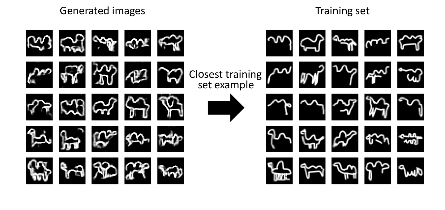
Figure 4-10. Closest matches of generated images from the training set

GAN Challenges

While GANs are a major breakthrough for generative modeling, they are also notoriously difficult to train. We will explore some of the most common problems encountered when training GANs in this section, then we will look at some adjustments to the GAN framework that remedy many of these problems.

Oscillating Loss

The loss of the discriminator and generator can start to oscillate wildly, rather than exhibiting long-term stability. Typically, there is some small oscillation of the loss between batches, but in the long term you should be looking for loss that stabilizes or gradually increases or decreases (see Figure 4-8), rather than erratically fluctuating, to ensure your GAN converges and improves over time. Figure 4-11 shows an example of a GAN where the loss of the discriminator and generator has started to spiral out of control, at around batch 1,400. It is difficult to establish if or when this might occur as vanilla GANs are prone to this kind of instability.

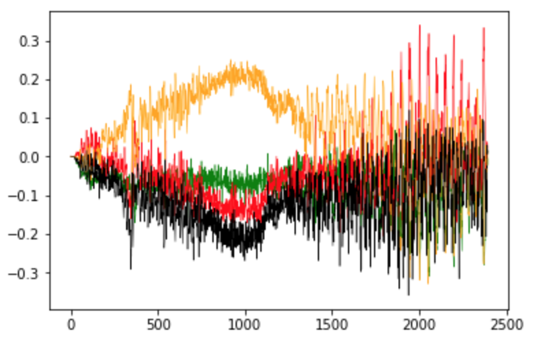
Figure 4-11. Oscillating loss in an unstable GAN

Mode Collapse

Mode collapse occurs when the generator finds a small number of samples that fool the discriminator and therefore isn’t able to produce any examples other than this limited set. Let’s think about how this might occur. Suppose we train the generator over several batches without updating the discriminator in between. The generator would be inclined to find a single observation (also known as a mode) that always fools the discriminator and would start to map every point in the latent input space to this observation. This means that the gradient of the loss function collapses to near 0. Even if we then try to retrain the discriminator to stop it being fooled by this one point, the generator will simply find another mode that fools the discriminator, since it has already become numb to its input and therefore has no incentive to diversify its output. The effect of mode collapse can be seen in Figure 4-12.

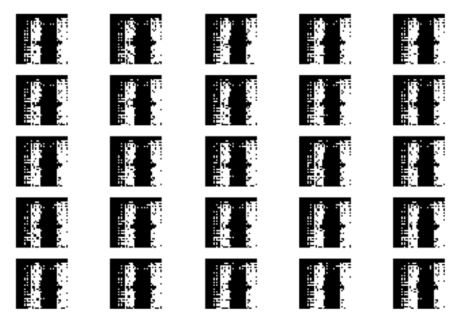
Figure 4-12. Mode collapse

Uninformative Loss

Since the deep learning model is compiled to minimize the loss function, it would be natural to think that the smaller the loss function of the generator, the better the quality of the images produced. However, since the generator is only graded against the current discriminator and the discriminator is constantly improving, we cannot compare the loss function evaluated at different points in the training process. Indeed, in Figure 4-8, the loss function of the generator actually increases over time, even though the quality of the images is clearly improving. This lack of correlation between the generator loss and image quality sometimes makes GAN training difficult to monitor.

Hyperparameters

As we have seen, even with simple GANs, there are a large number of hyperparameters to tune. As well as the overall architecture of both the discriminator and the generator, there are the parameters that govern the batch normalization, dropout, learning rate, activation layers, convolutional filters, kernel size, striding, batch size, and latent space size to consider. GANs are highly sensitive to very slight changes in all of these parameters, and finding a set of parameters that works is often a case of educated trial and error, rather than following an established set of guidelines.

This is why it is important to understand the inner workings of the GAN and know how to interpret the loss function—so that you can identify sensible adjustments to the hyperparameters that might improve the stability of the model.

Tackling the GAN Challenges

In recent years, several key advancements have drastically improved the overall stability of GAN models and diminished the likelihood of some of the problems listed earlier, such as mode collapse.

In the remainder of this chapter we shall explore two such advancements, the Wasserstein GAN (WGAN) and Wasserstein GAN–Gradient Penalty (WGAN-GP). Both are only minor adjustments to the framework we have explored thus far. The latter is now considered best practice for training the most sophisticated GANs available today.

Wasserstein GAN

The Wasserstein GAN was one of the first big steps toward stabilizing GAN training.⁴ With a few changes, the authors were able to show how to train GANs that have the following two properties (quoted from the paper):

• A meaningful loss metric that correlates with the generator’s convergence and sample quality

• Improved stability of the optimization process

Specifically, the paper introduces a new loss function for both the discriminator and the generator. Using this loss function instead of binary cross entropy results in a more stable convergence of the GAN. The mathematical explanation for this is beyond the scope of this book, but there are some excellent resources available online that explain the rationale behind switching to this loss function.

Let’s take a look at the definition of the Wasserstein loss function.

Wasserstein Loss

Let’s first remind ourselves of binary cross-entropy loss - the function that that we are currently using to train the discriminator and generator of the GAN:

Binary cross-entropy loss

$-\frac{1}{n}{\sum }_{i=1}^n(y_{i}log\left(p_i\right)+(1-y_i)log(1-p_i))$

To train the GAN discriminator D, we calculate the loss when comparing predictions for real images p_i=D(x_i) to the response y_i=1 and predictions for generated images p_i=D(G(z_i)) to the response y_i=0. Therefore for the GAN discriminator, minimizing the loss function can be written as follows:

GAN discriminator loss minimization

${min}_D-({𝔼}_{x\sim p_X}[logD\left(x\right)]+{𝔼}_{z\sim p_Z}[log(1-D(G\left(z\right)\left)\right)])$

To train the GAN generator G, we calculate the loss when comparing predictions for generated images p_i=D(G(z_i)) to the response y_i=1. Therefore for the GAN generator, minimizing the loss function can be written as follows:

GAN generator loss minimization

${min}_G-\left({𝔼}_{z\sim p_Z}[logD\left(G\right(z\left)\right)]\right)$

Now let’s compare this to the Wasserstein loss function.

First, the Wasserstein loss requires that we use y_i=1 and y_i=-1 as labels, rather than 1 and 0. We also remove the sigmoid activation from the final layer of the discriminator, so that predictions p_i are no longer constrained to fall in the range [0,1], but instead can now be any number in the range [–∞, ∞]. For this reason, the discriminator in a WGAN is usually referred to as a critic. The Wasserstein loss function is then defined as follows:

Wasserstein loss

$-\frac{1}{n}{\sum }_{i=1}^n\left(y_i{p}_i\right)$

To train the WGAN critic D, we calculate the loss when comparing predictions for a real images p_i=D(x_i) to the response y_i=1 and predictions for generated images p_i=D(G(z_i)) to the response y_i=-1. Therefore for the WGAN critic, minimizing the loss function can be written as follows:

WGAN critic loss minimization

${min}_D-({𝔼}_{x\sim p_X}\left[D\left(x\right)\right]-{𝔼}_{z\sim p_Z}\left[D\left(G\left(z\right)\right)\right])$

In other words, the WGAN critic tries to maximise the difference between its predictions for real images and generated images, with real images scoring higher.

To train the WGAN generator, we calculate the loss when comparing predictions for generated images p_i=D(G(z_i)) to the response y_i=1. Therefore for the WGAN generator, minimizing the loss function can be written as follows:

WGAN generator loss minimization

${min}_G-\left({𝔼}_{z\sim p_Z}\left[D\left(G\left(z\right)\right)\right]\right)$

When we compile the models that train the WGAN critic and generator, we can specify that we want to use the Wasserstein loss instead of the binary cross-entropy, as shown in Example 4-6. We also tend to use smaller learning rates for WGANs.

Example 4-6. Compiling the models that train the critic and generator

def wasserstein(y_true, y_pred):
    return -K.mean(y_true * y_pred)


critic.compile(
    optimizer= RMSprop(lr=0.00005)
    , loss = wasserstein
)

model.compile(
    optimizer= RMSprop(lr=0.00005)
    , loss = wasserstein
)

The Lipschitz Constraint

It may surprise you that we are now allowing the critic to output any number in the range [–∞, ∞], rather than applying a sigmoid function to restrict the output to the usual [0, 1] range. The Wasserstein loss can therefore be very large, which is unsettling—usually, large numbers in neural networks are to be avoided!

In fact, the authors of the WGAN paper show that for the Wasserstein loss function to work, we also need to place an additional constraint on the critic. Specifically, it is required that the critic is a 1-Lipschitz continuous function. Let’s pick this apart to understand what it means in more detail.

The critic is a function D that converts an image into a prediction. We say that this function is 1-Lipschitz if it satisfies the following inequality for any two input images, x₁ and x₂:

$$\frac{|D\left(x_1\right)-D\left(x_2\right)|}{|x_1-x_2|}\le 1$$

Here, x₁ – x₂ is the average pixelwise absolute difference between two images and $|D\left(x_1\right)-D\left(x_2\right)|$ is the absolute difference between the critic predictions. Essentially, we require a limit on the rate at which the predictions of the critic can change between two images (i.e., the absolute value of the gradient must be at most 1 everywhere). We can see this applied to a Lipschitz continuous 1D function in Figure 4-13—at no point does the line enter the cone, wherever you place the cone on the line. In other words, there is a limit on the rate at which the line can rise or fall at any point.

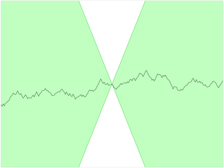
Figure 4-13. A Lipschitz continuous function—there exists a double cone such that wherever it is placed on the line, the function always remains entirely outside the cone⁵

For those who want to delve deeper into the mathematical rationale behind why the Wasserstein loss only works when this constraint is enforced, Jonathan Hui offers an excellent explanation.

Weight Clipping

In the WGAN paper, the authors show how it is possible to enforce the Lipschitz constraint by clipping the weights of the critic to lie within a small range, [–0.01, 0.01], after each training batch.

We can include this clipping process in our WGAN critic training function shown in Example 4-7.

Example 4-7. Training the critic of the WGAN

def train_critic(x_train, batch_size, clip_threshold):

    valid = np.ones((batch_size,1))
    fake = -np.ones((batch_size,1))

    # TRAIN ON REAL IMAGES
    idx = np.random.randint(0, x_train.shape[0], batch_size)
    true_imgs = x_train[idx]
    self.critic.train_on_batch(true_imgs, valid)

    # TRAIN ON GENERATED IMAGES
    noise = np.random.normal(0, 1, (batch_size, self.z_dim))
    gen_imgs = self.generator.predict(noise)
    self.critic.train_on_batch(gen_imgs, fake)

    for l in critic.layers:
        weights = l.get_weights()
        weights = [np.clip(w, -clip_threshold, clip_threshold) for w in weights]
        l.set_weights(weights)

Training the WGAN

When using the Wasserstein loss function, we should train the critic to convergence to ensure that the gradients for the generator update are accurate. This is in contrast to a standard GAN, where it is important not to let the discriminator get too strong, to avoid vanishing gradients.

Therefore, using the Wasserstein loss removes one of the key difficulties of training GANs—how to balance the training of the discriminator and generator. With WGANs, we can simply train the critic several times between generator updates, to ensure it is close to convergence. A typical ratio used is five critic updates to one generator update.

The training loop of the WGAN is shown in Example 4-8.

Example 4-8. Training the WGAN

for epoch in range(epochs):

    for _ in range(5):
        train_critic(x_train, batch_size = 128, clip_threshold = 0.01)

    train_generator(batch_size)

We have now covered all of the key differences between a standard GAN and a WGAN. To recap:

• A WGAN uses the Wasserstein loss.

• The WGAN is trained using labels of 1 for real and –1 for fake.

• There is no need for the sigmoid activation in the final layer of the WGAN critic.

• Clip the weights of the critic after each update.

• Train the critic multiple times for each update of the generator.

Analysis of the WGAN

You can train your own WGAN using code from the Jupyter notebook 04_02_wgan_cifar_train.ipynb in the book repository. This will train a WGAN to generate images of horses from the CIFAR-10 dataset, which we used in Chapter 2.

In Figure 4-14 we show some of the samples generated by the WGAN.

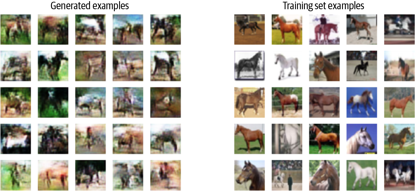
Figure 4-14. Examples from the generator of a WGAN trained on images of horses

Clearly, this is a much more difficult task than our previous ganimal example, but the WGAN has done a good job of establishing the key features of horse images (legs, sky, grass, brownness, shadow, etc.). As well as the images being in color, there are also many varying angles, shapes, and backgrounds for the WGAN to deal with in the training set. Therefore while the image quality isn’t yet perfect, we should be encouraged by the fact that our WGAN is clearly learning the high-level features that make up a color photograph of a horse.

One of the main criticisms of the WGAN is that since we are clipping the weights in the critic, its capacity to learn is greatly diminished. In fact, even in the original WGAN paper the authors write, “Weight clipping is a clearly terrible way to enforce a Lipschitz constraint.”

A strong critic is pivotal to the success of a WGAN, since without accurate gradients, the generator cannot learn how to adapt its weights to produce better samples.

Therefore, other researchers have looked for alternative ways to enforce the Lipschitz constraint and improve the capacity of the WGAN to learn complex features. We shall explore one such breakthrough in the next section.

WGAN-GP

One of the most recent extensions to the WGAN literature is the Wasserstein GAN–Gradient Penalty (WGAN-GP) framework.⁶

The WGAN-GP generator is defined and compiled in exactly the same way as the WGAN generator. It is only the definition and compilation of the critic that we need to change.

In total, there are three changes we need to make to our WGAN critic to convert it to a WGAN-GP critic:

• Include a gradient penalty term in the critic loss function.

• Don’t clip the weights of the critic.

• Don’t use batch normalization layers in the critic.

Let’s start by seeing how we can build the gradient penalty term into our loss function. In the paper introducing this variant, the authors propose an alternative way to enforce the Lipschitz constraint on the critic. Rather than clipping the weights of the critic, they show how the constraint can be enforced directly by including a term in the loss function that penalizes the model if the gradient norm of the critic deviates from 1. This is a much more natural way to achieve the constraint and results in a far more stable training process.

The Gradient Penalty Loss

Figure 4-15 is a diagram of the training process for the critic. If we compare this to the original discriminator training process from Figure 4-7, we can see that the key addition is the gradient penalty loss included as part of the overall loss function, alongside the Wasserstein loss from the real and fake images.

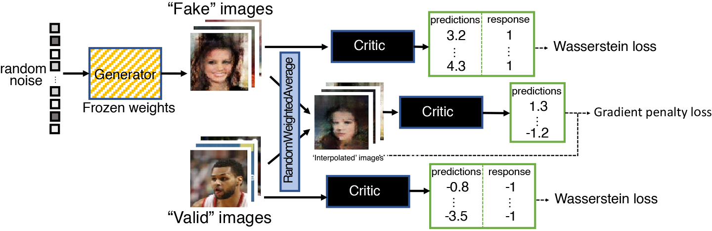
Figure 4-15. The WGAN-GP critic training process

The gradient penalty loss measures the squared difference between the norm of the gradient of the predictions with respect to the input images and 1. The model will naturally be inclined to find weights that ensure the gradient penalty term is minimized, thereby encouraging the model to conform to the Lipschitz constraint.

It is intractable to calculate this gradient everywhere during the training process, so instead the WGAN-GP evaluates the gradient at only a handful of points. To ensure a balanced mix, we use a set of interpolated images that lie at randomly chosen points along lines connecting the batch of real images to the batch of fake images pairwise, as shown in Figure 4-16.

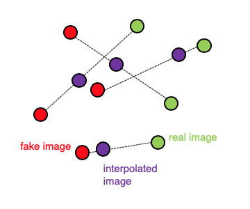
Figure 4-16. Interpolating between images

In Keras, we can create a RandomWeightedAverage layer to perform this interpolating operation, by inheriting from the built-in _Merge layer:

class RandomWeightedAverage(_Merge):
    def __init__(self, batch_size):
        super().__init__()
        self.batch_size = batch_size
    def _merge_function(self, inputs):
        alpha = K.random_uniform((self.batch_size, 1, 1, 1)) 
        return (alpha * inputs[0]) + ((1 - alpha) * inputs[1]) 

Each image in the batch gets a random number, between 0 and 1, stored as the vector alpha.

The layer returns the set of pixelwise interpolated images that lie along the lines connecting the real images (inputs[0]) to the fake images (inputs[1]), pairwise, weighted by the alpha value for each pair.

The gradient_penalty_loss function shown in Example 4-9 returns the squared difference between the gradient calculated at the interpolated points and 1.

Example 4-9. The gradient penalty loss function

def gradient_penalty_loss(y_true, y_pred, interpolated_samples):

    gradients = K.gradients(y_pred, interpolated_samples)[0] 

    gradient_l2_norm = K.sqrt(
        K.sum(
            K.square(gradients),
            axis=[1:len(gradients.shape)]
            )
        )
    ) 
    gradient_penalty = K.square(1 - gradient_l2_norm)
    return K.mean(gradient_penalty) 

The Keras gradients function calculates the gradients of the predictions for the interpolated images (y_pred) with respect to the input (interpolated_samples).

We calculate the L2 norm of this vector (i.e., its Euclidean length).

The function returns the squared distance between the L2 norm and 1.

Now that we have the RandomWeightedAverage layer that can interpolate between two images and the gradient_penalty_loss function that can calculate the gradient loss for the interpolated images, we can use both of these in the model compilation of the critic.

In the WGAN example, we compiled the critic directly, to predict if a given image was real or fake. To compile the WGAN-GP critic, we need to use the interpolated images in the loss function—however, Keras only permits a custom loss function with two parameters, the predictions and the true labels. To get around this issue, we use the Python partial function.

Example 4-10 shows the full compilation of the WGAN-GP critic in code.

Example 4-10. Compiling the WGAN-GP critic

from functools import partial

### COMPILE CRITIC MODEL

self.generator.trainable = False 

real_img = Input(shape=self.input_dim) 
z_disc = Input(shape=(self.z_dim,))
fake_img = self.generator(z_disc)

fake = self.critic(fake_img) 
valid = self.critic(real_img)

interpolated_img = RandomWeightedAverage(self.batch_size)([real_img, fake_img]) 
validity_interpolated = self.critic(interpolated_img)

partial_gp_loss = partial(self.gradient_penalty_loss,
                          interpolated_samples = interpolated_img) 
partial_gp_loss.__name__ = 'gradient_penalty' 

self.critic_model = Model(inputs=[real_img, z_disc],
                          outputs=[valid, fake, validity_interpolated]) 

self.critic_model.compile(
    loss=[self.wasserstein,self.wasserstein, partial_gp_loss]
    ,optimizer=Adam(lr=self.critic_learning_rate, beta_1=0.5)
    ,loss_weights=[1, 1, self.grad_weight]
    ) 

Freeze the weights of the generator. The generator forms part of the model that we are using to train the critic, as the interpolated images are now actively involved in the loss function, so this is required.

There are two inputs to the model: a batch of real images and a set of randomly generated numbers that are used to generate a batch of fake images.

The real and fake images are passed through the critic in order to calculate the Wasserstein loss.

The RandomWeightedAverage layer creates the interpolated images, which are then also passed through the critic.

Keras is expecting a loss function with only two inputs—the predictions and true labels—so we define a custom loss function, partial_gp_loss, using the Python partial function to pass the interpolated images through to our gradient_penalty_loss function.

Keras requires the function to be named.

The model that trains the critic is defined to have two inputs: the batch of real images and the random input that will generate the batch of fake images. The model has three outputs: 1 for the real images, –1 for the fake images, and a dummy 0 vector, which isn’t actually used but is required by Keras as every loss function must map to an output. Therefore we create the dummy 0 vector to map to the partial_gp_loss function.

We compile the critic with three loss functions: two Wasserstein losses for the real and fake images, and the gradient penalty loss. The overall loss is the sum of these three losses, with the gradient loss weighted by a factor of 10, in line with the recommendations from the original paper. We use the Adam optimizer, which is generally regarded to be the best optimizer for WGAN-GP models.

Batch Normalization in WGAN-GP

One last consideration we should note before building a WGAN-GP is that batch normalization shouldn’t be used in the critic. This is because batch normalization creates correlation between images in the same batch, which makes the gradient penalty loss less effective. Experiments have shown that WGAN-GPs can still produce excellent results even without batch normalization in the critic.

Analysis of WGAN-GP

Running the Jupyter notebook 04_03_wgangp_faces_train.ipynb in the book repository will train a WGAN-GP model on the CelebA dataset of celebrity faces.

First, let’s take a look at some uncurated example outputs from the generator, after 3,000 training batches (Figure 4-17).

Figure 4-17. WGAN-GP CelebA examples

Clearly the model has learned the significant high-level attributes of a face, and there is no sign of mode collapse.

We can also see how the loss functions of the model evolve over time (Figure 4-18)—the loss functions of both the discriminator and generator are highly stable and convergent.

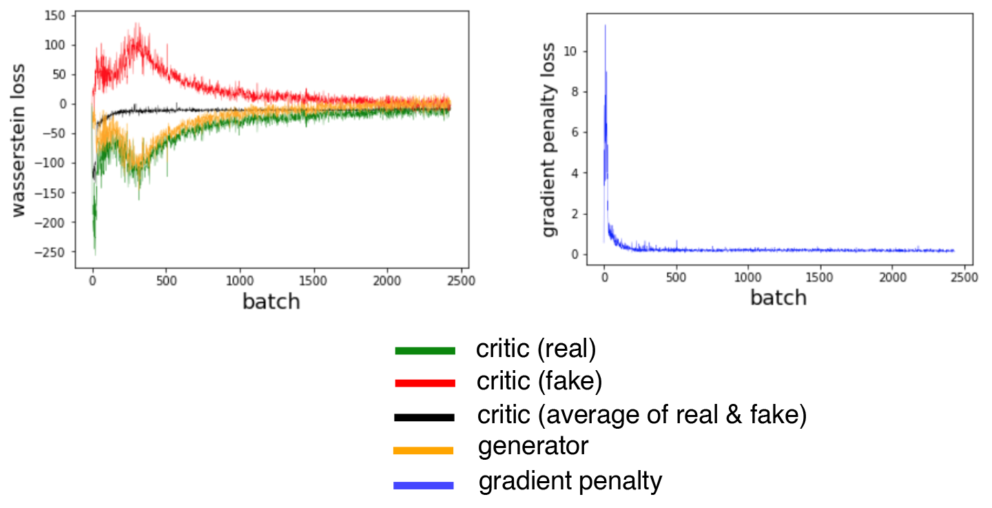
Figure 4-18. WGAN-GP loss

If we compare the WGAN-GP output to the VAE output from the previous chapter, we can see that the GAN images are generally sharper—especially the definition between the hair and the background. This is true in general; VAEs tend to produce softer images that blur color boundaries, whereas GANs are known to produce sharper, more well-defined images.

It is also true that GANs are generally more difficult to train than VAEs and take longer to reach a satisfactory quality. However, most of the state-of-the-art generative models today are GAN-based, as the rewards for training large-scale GANs on GPUs over a longer period of time are significant.

Summary

In this chapter we have explored three distinct flavors of generative adversarial networks, from the most fundamental vanilla GANs, through the Wasserstein GAN (WGAN), to the current state-of-the-art WGAN-GP models.

All GANs are characterized by a generator versus discriminator (or critic) architecture, with the discriminator trying to “spot the difference” between real and fake images and the generator aiming to fool the discriminator. By balancing how these two adversaries are trained, the GAN generator can gradually learn how to produce similar observations to those in the training set.

We saw how vanilla GANs can suffer from several problems, including mode collapse and unstable training, and how the Wasserstein loss function remedied many of these problems and made GAN training more predictable and reliable. The natural extension of the WGAN is the WGAN-GP, which places the 1-Lipschitz requirement at the heart of the training process by including a term in the loss function to pull the gradient norm toward 1.

Finally, we applied our new technique to the problem of face generation and saw how by simply choosing points from a standard normal distribution, we can generate new faces. This sampling process is very similar to a VAE, though the faces produced by a GAN are quite different—often sharper, with greater distinction between different parts of the image. When trained on a large number of GPUs, this property allows GANs to produce extremely impressive results and has taken the field of generative modeling to ever greater heights.

Overall, we have seen how the GAN framework is extremely flexible and able to be adapted to many interesting problem domains. We’ll look at one such application in the next chapter and explore how we can teach machines to paint.

¹ Ian Goodfellow, “NIPS 2016 Tutorial: Generative Adversarial Networks,” 21 December 2016, https://arxiv.org/abs/1701.00160v4.

² By happy coincidence, ganimals look exactly like camels.

³ Source: Augustus Odena et al., “Deconvolution and Checkerboard Artifacts, 17 October 2016, http://bit.ly/31MgHUQ.

⁴ Martin Arjovsky et al., “Wasserstein GAN,” 26 January 2017, https://arxiv.org/pdf/1701.07875.pdf.

⁵ Source: Wikipedia, http://bit.ly/2Xufwd8.

⁶ Ishaan Gulrajani et al., “Improved Training of Wasserstein GANs,” 31 March 2017, https://arxiv.org/abs/1704.00028.