Generative Deep Learning, 2nd Edition

Chapter 1. Generative Modeling

Chapter Goals

In this chapter you will:

• Learn the key differences between generative and discriminative models.

• Understand the desirable properties of a generative model through a simple example.

• Learn about the core probabilistic concepts that underpin generative models.

• Explore the different families of generative models.

• Clone the codebase that accompanies this book, so that you can get started building generative models!

This chapter is a general introduction to the field of generative modeling.

We will start with a gentle theoretical introduction to generative modeling and see how it is the natural counterpart to the more widely studied discriminative modeling. We will then establish a framework that describes the desirable properties that a good generative model should have. We will also lay out the core probabilistic concepts that are important to know, in order to fully appreciate how different approaches tackle the challenge of generative modeling.

This will lead us naturally to the penultimate section, which lays out the six broad families of generative models that dominate the field today. The final section explains how to get started with the codebase that accompanies this book.

What Is Generative Modeling?

Generative modeling can be broadly defined as follows:

Generative modeling is a branch of machine learning that involves training a model to produce new data that is similar to a given dataset.

What does this mean in practice? Suppose we have a dataset containing photos of horses. We can train a generative model on this dataset to capture the rules that govern the complex relationships between pixels in images of horses. Then we can sample from this model to create novel, realistic images of horses that did not exist in the original dataset. This process is illustrated in Figure 1-1.

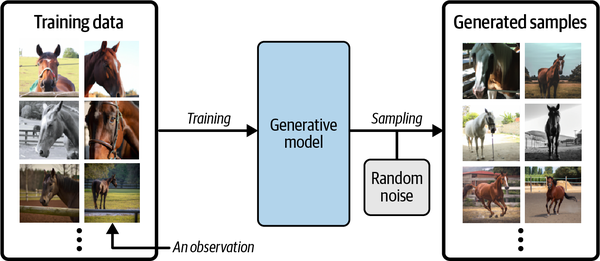
Figure 1-1. A generative model trained to generate realistic photos of horses

In order to build a generative model, we require a dataset consisting of many examples of the entity we are trying to generate. This is known as the training data, and one such data point is called an observation.

Each observation consists of many features. For an image generation problem, the features are usually the individual pixel values; for a text generation problem, the features could be individual words or groups of letters. It is our goal to build a model that can generate new sets of features that look as if they have been created using the same rules as the original data. Conceptually, for image generation this is an incredibly difficult task, considering the vast number of ways that individual pixel values can be assigned and the relatively tiny number of such arrangements that constitute an image of the entity we are trying to generate.

A generative model must also be probabilistic rather than deterministic, because we want to be able to sample many different variations of the output, rather than get the same output every time. If our model is merely a fixed calculation, such as taking the average value of each pixel in the training dataset, it is not generative. A generative model must include a random component that influences the individual samples generated by the model.

In other words, we can imagine that there is some unknown probabilistic distribution that explains why some images are likely to be found in the training dataset and other images are not. It is our job to build a model that mimics this distribution as closely as possible and then sample from it to generate new, distinct observations that look as if they could have been included in the original training set.

Generative Versus Discriminative Modeling

In order to truly understand what generative modeling aims to achieve and why this is important, it is useful to compare it to its counterpart, discriminative modeling. If you have studied machine learning, most problems you will have faced will have most likely been discriminative in nature. To understand the difference, let’s look at an example.

Suppose we have a dataset of paintings, some painted by Van Gogh and some by other artists. With enough data, we could train a discriminative model to predict if a given painting was painted by Van Gogh. Our model would learn that certain colors, shapes, and textures are more likely to indicate that a painting is by the Dutch master, and for paintings with these features, the model would upweight its prediction accordingly. Figure 1-2 shows the discriminative modeling process—note how it differs from the generative modeling process shown in Figure 1-1.

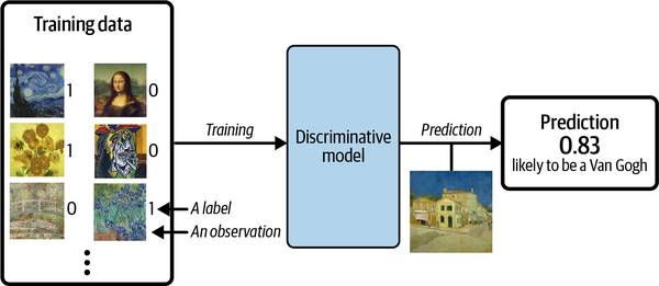
Figure 1-2. A discriminative model trained to predict if a given image is painted by Van Gogh

When performing discriminative modeling, each observation in the training data has a label. For a binary classification problem such as our artist discriminator, Van Gogh paintings would be labeled 1 and non–Van Gogh paintings labeled 0. Our model then learns how to discriminate between these two groups and outputs the probability that a new observation has label 1—i.e., that it was painted by Van Gogh.

In contrast, generative modeling doesn’t require the dataset to be labeled because it concerns itself with generating entirely new images, rather than trying to predict a label of a given image.

Let’s define these types of modeling formally, using mathematical notation:

Discriminative modeling estimates $p\left(y\right|𝐱)$.

That is, discriminative modeling aims to model the probability of a label $y$ given some observation $𝐱$.

Generative modeling estimates $p\left(𝐱\right)$.

That is, generative modeling aims to model the probability of observing an observation $𝐱$. Sampling from this distribution allows us to generate new observations.

Conditional Generative Models

Note that we can also build a generative model to model the conditional probability $p\left(𝐱\right|y)$—the probability of seeing an observation $𝐱$ with a specific label $y$.

For example, if our dataset contains different types of fruit, we could tell our generative model to specifically generate an image of an apple.

An important point to note is that even if we were able to build a perfect discriminative model to identify Van Gogh paintings, it would still have no idea how to create a painting that looks like a Van Gogh. It can only output probabilities against existing images, as this is what it has been trained to do. We would instead need to train a generative model and sample from this model to generate images that have a high chance of belonging to the original training dataset.

The Rise of Generative Modeling

Until recently, discriminative modeling has been the driving force behind most progress in machine learning. This is because for any discriminative problem, the corresponding generative modeling problem is typically much more difficult to tackle. For example, it is much easier to train a model to predict if a painting is by Van Gogh than it is to train a model to generate a Van Gogh–style painting from scratch. Similarly, it is much easier to train a model to predict if a page of text was written by Charles Dickens than it is to build a model to generate a set of paragraphs in the style of Dickens. Until recently, most generative challenges were simply out of reach and many doubted that they could ever be solved. Creativity was considered a purely human capability that couldn’t be rivaled by AI.

However, as machine learning technologies have matured, this assumption has gradually weakened. In the last 10 years many of the most interesting advancements in the field have come through novel applications of machine learning to generative modeling tasks. For example, Figure 1-3 shows the striking progress that has already been made in facial image generation since 2014.

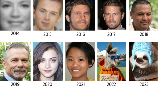
Figure 1-3. Face generation using generative modeling has improved significantly over the last decade (adapted from Brundage et al., 2018)¹

As well as being easier to tackle, discriminative modeling has historically been more readily applicable to practical problems across industry than generative modeling. For example, a doctor may benefit from a model that predicts if a given retinal image shows signs of glaucoma, but wouldn’t necessarily benefit from a model that can generate novel pictures of the back of an eye.

However, this is also starting to change, with the proliferation of companies offering generative services that target specific business problems. For example, it is now possible to access APIs that generate original blog posts given a particular subject matter, produce a variety of images of your product in any setting you desire, or write social media content and ad copy to match your brand and target message. There are also clear positive applications of generative AI for industries such as game design and cinematography, where models trained to output video and music are beginning to add value.

Generative Modeling and AI

As well as the practical uses of generative modeling (many of which are yet to be discovered), there are three deeper reasons why generative modeling can be considered the key to unlocking a far more sophisticated form of artificial intelligence that goes beyond what discriminative modeling alone can achieve.

Firstly, purely from a theoretical point of view, we shouldn’t limit our machine training to simply categorizing data. For completeness, we should also be concerned with training models that capture a more complete understanding of the data distribution, beyond any particular label. This is undoubtedly a more difficult problem to solve, due to the high dimensionality of the space of feasible outputs and the relatively small number of creations that we would class as belonging to the dataset. However, as we shall see, many of the same techniques that have driven development in discriminative modeling, such as deep learning, can be utilized by generative models too.

Secondly, as we shall see in Chapter 12, generative modeling is now being used to drive progress in other fields of AI, such as reinforcement learning (the study of teaching agents to optimize a goal in an environment through trial and error). Suppose we want to train a robot to walk across a given terrain. A traditional approach would be to run many experiments where the agent tries out different strategies in the terrain, or a computer simulation of the terrain. Over time the agent would learn which strategies are more successful than others and therefore gradually improve. A challenge with this approach is that it is fairly inflexible because it is trained to optimize the policy for one particular task. An alternative approach that has recently gained traction is to instead train the agent to learn a world model of the environment using a generative model, independent of any particular task. The agent can quickly adapt to new tasks by testing strategies in its own world model, rather than in the real environment, which is often computationally more efficient and does not require retraining from scratch for each new task.

Finally, if we are to truly say that we have built a machine that has acquired a form of intelligence that is comparable to a human’s, generative modeling must surely be part of the solution. One of the finest examples of a generative model in the natural world is the person reading this book. Take a moment to consider what an incredible generative model you are. You can close your eyes and imagine what an elephant would look like from any possible angle. You can imagine a number of plausible different endings to your favorite TV show, and you can plan your week ahead by working through various futures in your mind’s eye and taking action accordingly. Current neuroscientific theory suggests that our perception of reality is not a highly complex discriminative model operating on our sensory input to produce predictions of what we are experiencing, but is instead a generative model that is trained from birth to produce simulations of our surroundings that accurately match the future. Some theories even suggest that the output from this generative model is what we directly perceive as reality. Clearly, a deep understanding of how we can build machines to acquire this ability will be central to our continued understanding of the workings of the brain and general artificial intelligence.

Our First Generative Model

With this in mind, let’s begin our journey into the exciting world of generative modeling. To begin with, we’ll look at a toy example of a generative model and introduce some of the ideas that will help us to work through the more complex architectures that we will encounter later in the book.

Hello World!

Let’s start by playing a generative modeling game in just two dimensions. I have chosen a rule that has been used to generate the set of points $𝐗$ in Figure 1-4. Let’s call this rule $p_{data}$. Your challenge is to choose a different point $𝐱=(x_1,x_2)$ in the space that looks like it has been generated by the same rule.

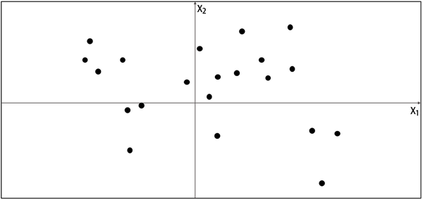
Figure 1-4. A set of points in two dimensions, generated by an unknown rule $p_{data}$

Where did you choose? You probably used your knowledge of the existing data points to construct a mental model, $p_{model}$, of whereabouts in the space the point is more likely to be found. In this respect, $p_{model}$ is an estimate of $p_{data}$. Perhaps you decided that $p_{model}$ should look like Figure 1-5—a rectangular box where points may be found, and an area outside of the box where there is no chance of finding any points.

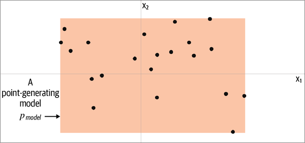
Figure 1-5. The orange box, $p_{model}$, is an estimate of the true data-generating distribution, $p_{data}$

To generate a new observation, you can simply choose a point at random within the box, or more formally, sample from the distribution $p_{model}$. Congratulations, you have just built your first generative model! You have used the training data (the black points) to construct a model (the orange region) that you can easily sample from to generate other points that appear to belong to the training set.

Let’s now formalize this thinking into a framework that can help us understand what generative modeling is trying to achieve.

The Generative Modeling Framework

We can capture our motivations and goals for building a generative model in the following framework.

The Generative Modeling Framework

• We have a dataset of observations $𝐗$.

• We assume that the observations have been generated according to some unknown distribution, $p_{data}$.

• We want to build a generative model $p_{model}$ that mimics $p_{data}$. If we achieve this goal, we can sample from $p_{model}$ to generate observations that appear to have been drawn from $p_{data}$.

• Therefore, the desirable properties of $p_{model}$ are:

  Accuracy

  If $p_{model}$ is high for a generated observation, it should look like it has been drawn from $p_{data}$. If $p_{model}$ is low for a generated observation, it should not look like it has been drawn from $p_{data}$.

  Generation

  It should be possible to easily sample a new observation from $p_{model}$.

  Representation

  It should be possible to understand how different high-level features in the data are represented by $p_{model}$.

Let’s now reveal the true data-generating distribution, $p_{data}$, and see how the framework applies to this example. As we can see from Figure 1-6, the data-generating rule is simply a uniform distribution over the land mass of the world, with no chance of finding a point in the sea.

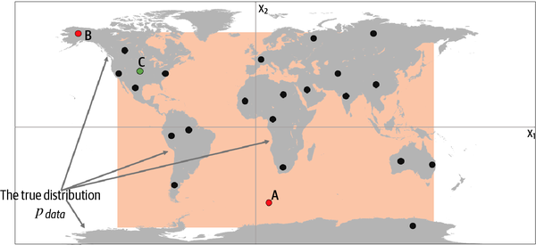
Figure 1-6. The orange box, $p_{model}$, is an estimate of the true data-generating distribution, $p_{data}$ (the gray area)

Clearly, our model, $p_{model}$, is an oversimplification of $p_{data}$. We can inspect points A, B, and C to understand the successes and failures of our model in terms of how accurately it mimics $p_{data}$:

• Point A is an observation that is generated by our model but does not appear to have been generated by $p_{data}$ as it’s in the middle of the sea.

• Point B could never have been generated by $p_{model}$ as it sits outside the orange box. Therefore, our model has some gaps in its ability to produce observations across the entire range of potential possibilities.

• Point C is an observation that could be generated by $p_{model}$ and also by $p_{data}$.

Despite its shortcomings, the model is easy to sample from, because it is simply a uniform distribution over the orange box. We can easily choose a point at random from inside this box, in order to sample from it.

Also, we can certainly say that our model is a simple representation of the underlying complex distribution that captures some of the underlying high-level features. The true distribution is separated into areas with lots of land mass (continents) and those with no land mass (the sea). This is a high-level feature that is also true of our model, except we have one large continent, rather than many.

This example has demonstrated the fundamental concepts behind generative modeling. The problems we will be tackling in this book will be far more complex and high-dimensional, but the underlying framework through which we approach the problem will be the same.

Representation Learning

It is worth delving a little deeper into what we mean by learning a representation of the high-dimensional data, as it is a topic that will recur throughout this book.

Suppose you wanted to describe your appearance to someone who was looking for you in a crowd of people and didn’t know what you looked like. You wouldn’t start by stating the color of pixel 1 of a photo of you, then pixel 2, then pixel 3, etc. Instead, you would make the reasonable assumption that the other person has a general idea of what an average human looks like, then amend this baseline with features that describe groups of pixels, such as I have very blond hair or I wear glasses. With no more than 10 or so of these statements, the person would be able to map the description back into pixels to generate an image of you in their head. The image wouldn’t be perfect, but it would be a close enough likeness to your actual appearance for them to find you among possibly hundreds of other people, even if they’ve never seen you before.

This is the core idea behind representation learning. Instead of trying to model the high-dimensional sample space directly, we describe each observation in the training set using some lower-dimensional latent space and then learn a mapping function that can take a point in the latent space and map it to a point in the original domain. In other words, each point in the latent space is a representation of some high-dimensional observation.

What does this mean in practice? Let’s suppose we have a training set consisting of grayscale images of biscuit tins (Figure 1-7).

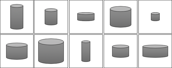
Figure 1-7. The biscuit tin dataset

To us, it is obvious that there are two features that can uniquely represent each of these tins: the height and width of the tin. That is, we can convert each image of a tin to a point in a latent space of just two dimensions, even though the training set of images is provided in high-dimensional pixel space. Notably, this means that we can also produce images of tins that do not exist in the training set, by applying a suitable mapping function $f$ to a new point in the latent space, as shown in Figure 1-8.

Realizing that the original dataset can be described by the simpler latent space is not so easy for a machine—it would first need to establish that height and width are the two latent space dimensions that best describe this dataset, then learn the mapping function $f$ that can take a point in this space and map it to a grayscale biscuit tin image. Machine learning (and specifically, deep learning) gives us the ability to train machines that can find these complex relationships without human guidance.

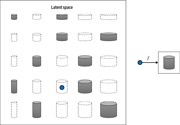
Figure 1-8. The 2D latent space of biscuit tins and the function $f$ that maps a point in the latent space back to the original image domain

One of the benefits of training models that utilize a latent space is that we can perform operations that affect high-level properties of the image by manipulating its representation vector within the more manageable latent space. For example, it is not obvious how to adjust the shading of every single pixel to make an image of a biscuit tin taller. However, in the latent space, it’s simply a case of increasing the height latent dimension, then applying the mapping function to return to the image domain. We shall see an explicit example of this in the next chapter, applied not to biscuit tins but to faces.

The concept of encoding the training dataset into a latent space so that we can sample from it and decode the point back to the original domain is common to many generative modeling techniques, as we shall see in later chapters of this book. Mathematically speaking, encoder-decoder techniques try to transform the highly nonlinear manifold on which the data lies (e.g., in pixel space) into a simpler latent space that can be sampled from, so that it is likely that any point in the latent space is the representation of a well-formed image, as shown in Figure 1-9.

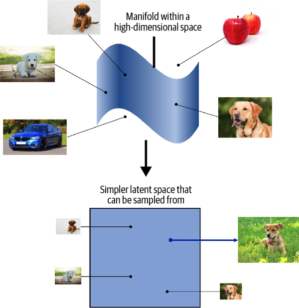
Figure 1-9. The dog manifold in high-dimensional pixel space is mapped to a simpler latent space that can be sampled from

Core Probability Theory

We have already seen that generative modeling is closely connected to statistical modeling of probability distributions. Therefore, it now makes sense to introduce some core probabilistic and statistical concepts that will be used throughout this book to explain the theoretical background of each model.

If you have never studied probability or statistics, don’t worry. To build many of the deep learning models that we shall see later in this book, it is not essential to have a deep understanding of statistical theory. However, to gain a full appreciation of the task that we are trying to tackle, it’s worth trying to build up a solid understanding of basic probabilistic theory. This way, you will have the foundations in place to understand the different families of generative models that will be introduced later in this chapter.

As a first step, we shall define five key terms, linking each one back to our earlier example of a generative model that models the world map in two dimensions:

Sample space

The sample space is the complete set of all values an observation $𝐱$ can take.

Note

In our previous example, the sample space consists of all points of latitude and longitude $𝐱=(x_1,x_2)$ on the world map. For example, $𝐱$ = (40.7306, –73.9352) is a point in the sample space (New York City) that belongs to the true data-generating distribution. $𝐱$ = (11.3493, 142.1996) is a point in the sample space that does not belong to the true data-generating distribution (it’s in the sea).

Probability density function

A probability density function (or simply density function) is a function $p\left(𝐱\right)$ that represents the relative likelihood of a continuous random variable falling within different intervals, with the integral of $p\left(𝐱\right)$ over the entire range of possible values being equal to 1.

Note

In the world map example, the density function of our generative model is 0 outside of the orange box and constant inside of the box, so that the integral of the density function over the entire sample space equals 1.

While there is only one true density function $p_{data}\left(𝐱\right)$ that is assumed to have generated the observable dataset, there are infinitely many density functions $p_{model}\left(𝐱\right)$ that we can use to estimate $p_{data}\left(𝐱\right)$.

Parametric modeling

Parametric modeling is a technique that we can use to structure our approach to finding a suitable $p_{model}\left(𝐱\right)$. A parametric model is a family of density functions $p_{\theta }\left(𝐱\right)$ that can be described using a finite number of parameters, $\theta$.

Note

If we assume a uniform distribution as our model family, then the set all possible boxes we could draw on Figure 1-5 is an example of a parametric model. In this case, there are four parameters: the coordinates of the bottom-left $({\theta }_1,{\theta }_2)$ and top-right $({\theta }_3,{\theta }_4)$ corners of the box.

Thus, each density function $p_{\theta }\left(𝐱\right)$ in this parametric model (i.e., each box) can be uniquely represented by four numbers, $\theta =({\theta }_1,{\theta }_2,{\theta }_3,{\theta }_4)$ .

Likelihood

The likelihood $ℒ\left(\theta \right|𝐱)$ of a parameter set $\theta$ is a function that measures the plausibility of $\theta$, given some observed point $𝐱$. It is defined as follows:

$$ℒ\left(\theta \right|𝐱)=p_{\theta }\left(𝐱\right)$$

That is, the likelihood of $\theta$ given some observed point $𝐱$ is defined to be the value of the density function parameterized by $\theta$, at the point $𝐱$. If we have a whole dataset $𝐗$ of independent observations, then we can write:

$$ℒ\left(\theta \right|𝐗)=\prod _{𝐱\in 𝐗}{p}_{\theta }\left(𝐱\right)$$

Note

In the world map example, an orange box that only covered the left half of the map would have a likelihood of 0—it couldn’t possibly have generated the dataset, as we have observed points in the right half of the map. The orange box in Figure 1-5 has a positive likelihood, as the density function is positive for all data points under this model.

Since the product of a large number of terms between 0 and 1 can be quite computationally difficult to work with, we often use the log-likelihood ℓ instead:

$$\ell \left(\theta \right|𝐗)=\sum _{𝐱\in 𝐗}log{p}_{\theta }\left(𝐱\right)$$

There are statistical reasons why the likelihood is defined in this way, but we can also see that this definition intuitively makes sense. The likelihood of a set of parameters $\theta$ is defined to be the probability of seeing the data if the true data-generating distribution was the model parameterized by $\theta$.

Warning

Note that the likelihood is a function of the parameters, not the data. It should not be interpreted as the probability that a given parameter set is correct—in other words, it is not a probability distribution over the parameter space (i.e., it doesn’t sum/integrate to 1, with respect to the parameters).

It makes intuitive sense that the focus of parametric modeling should be to find the optimal value $\widehat{\theta }$ of the parameter set that maximizes the likelihood of observing the dataset $𝐗$.

Maximum likelihood estimation

Maximum likelihood estimation is the technique that allows us to estimate $\widehat{\theta }$—the set of parameters $\theta$ of a density function $p_{\theta }\left(𝐱\right)$ that is most likely to explain some observed data $𝐗$. More formally:

$$\widehat{\theta }=\underset{\theta }{argmax}\ell \left(\theta \right|𝐗)$$

$\widehat{\theta }$ is also called the maximum likelihood estimate (MLE).

Note

In the world map example, the MLE is the smallest rectangle that still contains all of the points in the training set.

Neural networks typically minimize a loss function, so we can equivalently talk about finding the set of parameters that minimize the negative log-likelihood:

$$\widehat{\theta }=\underset{\theta }{argmin}\left(-\ell \left(\theta \right|𝐗)\right)=\underset{\theta }{argmin}\left(-log{p}_{\theta }\left(𝐗\right)\right)$$

Generative modeling can be thought of as a form of maximum likelihood estimation, where the parameters $\theta$ are the weights of the neural networks contained in the model. We are trying to find the values of these parameters that maximize the likelihood of observing the given data (or equivalently, minimize the negative log-likelihood).

However, for high-dimensional problems, it is generally not possible to directly calculate $p_{\theta }\left(𝐱\right)$—it is intractable. As we shall see in the next section, different families of generative models take different approaches to tackling this problem.

Generative Model Taxonomy

While all types of generative models ultimately aim to solve the same task, they all take slightly different approaches to modeling the density function $p_{\theta }\left(𝐱\right)$. Broadly speaking, there are three possible approaches:

1. Explicitly model the density function, but constrain the model in some way, so that the density function is tractable (i.e., it can be calculated).

2. Explicitly model a tractable approximation of the density function.

3. Implicitly model the density function, through a stochastic process that directly generates data.

These are shown in Figure 1-10 as a taxonomy, alongside the six families of generative models that we will explore in Part II of this book. Note that these families are not mutually exclusive—there are many examples of models that are hybrids between two different kinds of approaches. You should think of the families as different general approaches to generative modeling, rather than explicit model architectures.

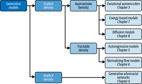
Figure 1-10. A taxonomy of generative modeling approaches

The first split that we can make is between models where the probability density function $p\left(𝐱\right)$ is modeled explicitly and those where it is modeled implicitly.

Implicit density models do not aim to estimate the probability density at all, but instead focus solely on producing a stochastic process that directly generates data. The best-known example of an implicit generative model is a generative adversarial network. We can further split explicit density models into those that directly optimize the density function (tractable models) and those that only optimize an approximation of it.

Tractable models place constraints on the model architecture, so that the density function has a form that makes it easy to calculate. For example, autoregressive models impose an ordering on the input features, so that the output can be generated sequentially—e.g., word by word, or pixel by pixel. Normalizing flow models apply a series of tractable, invertible functions to a simple distribution, in order to generate more complex distributions.

Approximate density models include variational autoencoders, which introduce a latent variable and optimize an approximation of the joint density function. Energy-based models also utilize approximate methods, but do so via Markov chain sampling, rather than variational methods. Diffusion models approximate the density function by training a model to gradually denoise a given image that has been previously corrupted.

A common thread that runs through all of the generative model family types is deep learning. Almost all sophisticated generative models have a deep neural network at their core, because they can be trained from scratch to learn the complex relationships that govern the structure of the data, rather than having to be hardcoded with information a priori. We’ll explore deep learning in Chapter 2, with practical examples of how to get started building your own deep neural networks.

The Generative Deep Learning Codebase

The final section of this chapter will get you set up to start building generative deep learning models by introducing the codebase that accompanies this book.

Tip

Many of the examples in this book are adapted from the excellent open source implementations that are available through the Keras website. I highly recommend you check out this resource, as new models and examples are constantly being added.

Cloning the Repository

To get started, you’ll first need to clone the Git repository. Git is an open source version control system and will allow you to copy the code locally so that you can run the notebooks on your own machine, or in a cloud-based environment. You may already have this installed, but if not, follow the instructions relevant to your operating system.

To clone the repository for this book, navigate to the folder where you would like to store the files and type the following into your terminal:

git clone https://github.com/davidADSP/Generative_Deep_Learning_2nd_Edition.git

You should now be able to see the files in a folder on your machine.

Using Docker

The codebase for this book is intended to be used with Docker, a free containerization technology that makes getting started with a new codebase extremely easy, regardless of your architecture or operating system. If you have never used Docker, don’t worry—there is a description of how to get started in the README file in the book repository.

Running on a GPU

If you don’t have access to your own GPU, that’s also no problem! All of the examples in this book will train on a CPU, though this will take longer than if you use a GPU-enabled machine. There is also a section in the README about setting up a Google Cloud environment that gives you access to a GPU on a pay-as-you-go basis.

Summary

This chapter introduced the field of generative modeling, an important branch of machine learning that complements the more widely studied discriminative modeling. We discussed how generative modeling is currently one of the most active and exciting areas of AI research, with many recent advances in both theory and applications.

We started with a simple toy example and saw how generative modeling ultimately focuses on modeling the underlying distribution of the data. This presents many complex and interesting challenges, which we summarized into a framework for understanding the desirable properties of any generative model.

We then walked through the key probabilistic concepts that will help to fully understand the theoretical foundations of each approach to generative modeling and laid out the six different families of generative models that we will explore in Part II of this book. We also saw how to get started with the Generative Deep Learning codebase, by cloning the repository.

In Chapter 2, we will begin our exploration of deep learning and see how to use Keras to build models that can perform discriminative modeling tasks. This will give us the necessary foundation to tackle generative deep learning problems in later chapters.

¹ Miles Brundage et al., “The Malicious Use of Artificial Intelligence: Forecasting, Prevention, and Mitigation,” February 20, 2018, https://www.eff.org/files/2018/02/20/malicious_ai_report_final.pdf.