Generative AI on AWS

Chapter 4. Memory and Compute Optimizations

In Chapter 3, you explored best practices for experimenting with and selecting a foundation model for your use case. The next step is usually to customize the model to your specific needs and datasets. This could include adapting the model to your datasets using a technique called fine-tuning, which you will explore in more detail in Chapter 5. When training or fine-tuning large foundation models, you often face compute challenges—in particular, how to fit large models into GPU memory.

In this chapter, you will explore techniques that help overcome memory limitations. You will learn how to apply quantization and distributed training to minimize the required GPU RAM, and how to scale model training horizontally across multiple GPUs for larger models.

For example, the original 40 billion-parameter Falcon model was trained on a cluster of 48 ml.p4d.24xlarge Amazon SageMaker instances consisting of 384 NVIDIA A100 GPUs, 15TB of GPU RAM, and 55TB of CPU RAM. A more recent version of Falcon was trained on a cluster of 392 ml.p4d.24xlarge SageMaker instances consisting of 3,136 NVIDIA A100 GPUs, 125TB of GPU RAM, and 450TB of CPU RAM. The size and complexity of the Falcon model requires a cluster of GPUs, but also benefits from quantization, as you will see next.

Memory Challenges

One of the most common issues you’ll encounter when you try to train or fine-tune foundation models is running out of memory. If you’ve ever tried training or even just loading your model on NVIDIA GPUs, the error message in Figure 4-1 might look familiar.

Figure 4-1. CUDA out-of-memory error

CUDA, short for Compute Unified Device Architecture, is a collection of libraries and tools developed for NVIDIA GPUs to boost performance on common deep-learning operations, including matrix multiplication, among many others. Deep-learning libraries such as PyTorch and TensorFlow use CUDA extensively to handle the low-level, hardware-specific details, including data movement between CPU and GPU memory. As modern generative models contain multiple billions of parameters, you have likely encountered this out-of-memory error during development while loading and testing a model in your research environment.

A single-model parameter, at full 32-bit precision, is represented by 4 bytes. Therefore, a 1-billion-parameter model requires 4 GB of GPU RAM just to load the model into GPU RAM at full precision. If you want to also train the model, you need more GPU memory to store the states of the numerical optimizer, gradients, and activations, as well as any temporary variables used by your functions, as shown in Table 4-1.

Table 4-1. Additional RAM needed to train a model

States	Bytes per parameter
Model parameters (weights)	4 bytes per parameter
Adam optimizer (2 states)	8 bytes per parameter
Gradients	4 bytes per parameter
Activations and temp memory (variable size)	8 bytes per parameter (high-end estimate)
TOTAL	= 4 + 20 bytes per parameter

Tip

When you experiment with training a model, it’s recommended that you start with batch_size=1 to find the memory boundaries of the model with just a single training example. You can then incrementally increase the batch size until you hit the CUDA out-of-memory error. This will determine the maximum batch size for the model and dataset. A larger batch size can often speed up your model training.

These additional components lead to approximately 12–20 extra bytes of GPU memory per model parameter. For example, to train a 1-billion-parameter model, you will need approximately 24 GB of GPU RAM at 32-bit full precision, six times the memory compared to just 4 GB of GPU RAM for loading the model, as shown in Figure 4-2.

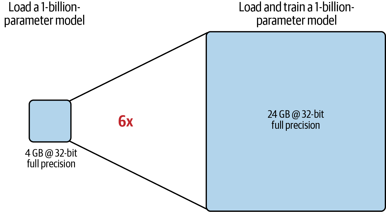
Figure 4-2. Comparison of approximate GPU RAM needed to load versus load and train a 1-billion-parameter model at 32-bit full precision

It’s worth noting that the NVIDIA A100 and H100, used at the time of this writing, only support up to 80 GB of GPU RAM. And since you likely want to train models larger than 1 billion parameters, you’ll need to find a workaround, such as quantizing your model.

AWS has also developed purpose-built ML accelerators, AWS Trainium, for high-performance and cost-efficient training of 100B+ parameter generative AI models. You can leverage AWS Trainium chips through the Trn1 instance family. The largest Trn1 instance, at the time of this writing, is powered by 16 AWS Trainium chips and has 512 GB of shared accelerator memory. In addition, Trn1 instances are optimized for quantization and distributed model training, and they support a wide range of data types.

Quantization is a popular way to convert your model parameters from 32-bit precision down to 16-bit precision—or even 8-bit or 4-bit. By quantizing your model weights from 32-bit full precision down to 16-bit half precision, you can quickly reduce your 1-billion-parameter-model memory requirement down 50% to only 2 GB for loading and 12 GB for training.

But before we dive into quantization, let’s explore common data types for model training and discuss numerical precision.

Data Types and Numerical Precision

The following are the various data types used by PyTorch and TensorFlow: fp32 for 32-bit full precision, fp16 for 16-bit half-precision, and int8 for 8-bit integer precision.

More recently, bfloat16 has become a popular alternative to fp16 for 16-bit precision in more-modern generative AI models. bfloat16 (or bf16) is short for “brain floating point 16” as it was developed at Google Brain. Compared to fp16, bfloat16 has a greater dynamic range with 8 bits for the exponent and can therefore represent a wide range of values that we find in generative AI models.

Let’s discuss how these data types compare and why bfloat16 is a popular choice for 16-bit quantization.

Suppose you want to store pi to 20 decimal places (3.14159265358979323846) using full 32-bit precision. Remember that floating point numbers are stored as a series of bits consisting of only 0s and 1s. Numbers are stored in 32-bits using 1 bit for the sign (negative or positive), 8 bits for the exponent (representing the dynamic range), and 23 bits for the fraction, also called the mantissa or significand, which represents the precision of the number. Table 4-2 shows how fp32 represents the value of pi.

Table 4-2. fp32 representing pi

Sign	Exponent	Fraction (mantissa/significand)
1 bit 0	8 bits 10000000	23 bits 10010010000111111011011

fp32 can represent numbers in a range from –3e38 to +3e38. The following PyTorch code shows how to print the data type information for fp32:

import torch
torch.finfo(torch.float32)

The output is:

finfo(resolution=1e-06, min=-3.40282e+38, max=3.40282e+38, eps=1.19209e-07, 
smallest_normal=1.17549e-38, tiny=1.17549e-38, dtype=float32)

Storing a real number in 32 bits will actually cause a slight loss in precision. You can see this by storing pi as an fp32 data type and then printing the value of the tensor to 20 decimal places using Tensor.item():

pi = 3.14159265358979323846
pi_fp32 = torch.tensor(pi, dtype=torch.float32)
print('%.20f' % pi_fp32.item())

The output is:

3.14159274101257324219

You can see the slight loss in precision if you compare this value to the real value of pi, which starts with 3.14159265358979323846. This slight loss in precision is due to the conversion into the fp32 number range, as depicted in Figure 4-3.

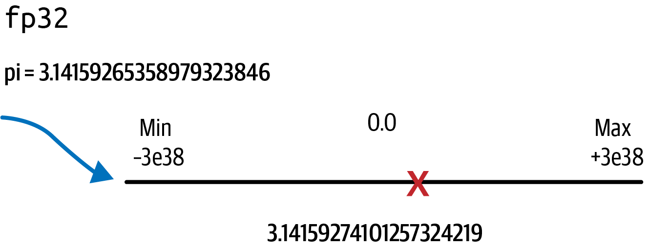
Figure 4-3. fp32 projecting pi into the range from –3e38 to +3e38

You can also print the memory consumption:

def show_memory_comsumption(tensor):
    memory_bytes = tensor.element_size() * tensor.numel()
    print("Tensor memory consumption:", memory_bytes, "bytes")
show_memory_comsumption(pi_fp32)

The output is:

Tensor memory consumption: 4 bytes

Now that you’ve explored data types and numerical representations, let’s move on and discuss how quantization can help you reduce the memory footprint required to load and train your multibillion-parameter model.

Quantization

When you try to train a multibillion-parameter model at 32-bit full precision, you will quickly hit the limit of a single NVIDIA A100 or H100 GPU with only 80 GB of GPU RAM. Therefore, you will almost always need to use quantization when using a single GPU.

Quantization reduces the memory needed to load and train a model by reducing the precision of the model weights. Quantization converts your model parameters from 32-bit precision down to 16-bit precision—or even 8-bit or 4-bit.

By quantizing your model weights from 32-bit full-precision down to 16-bit or 8-bit precision, you can quickly reduce your 1-billion-parameter-model memory requirement down 50% to only 2 GB, or even down 75% to just 1 GB for loading, as shown in Figure 4-4.

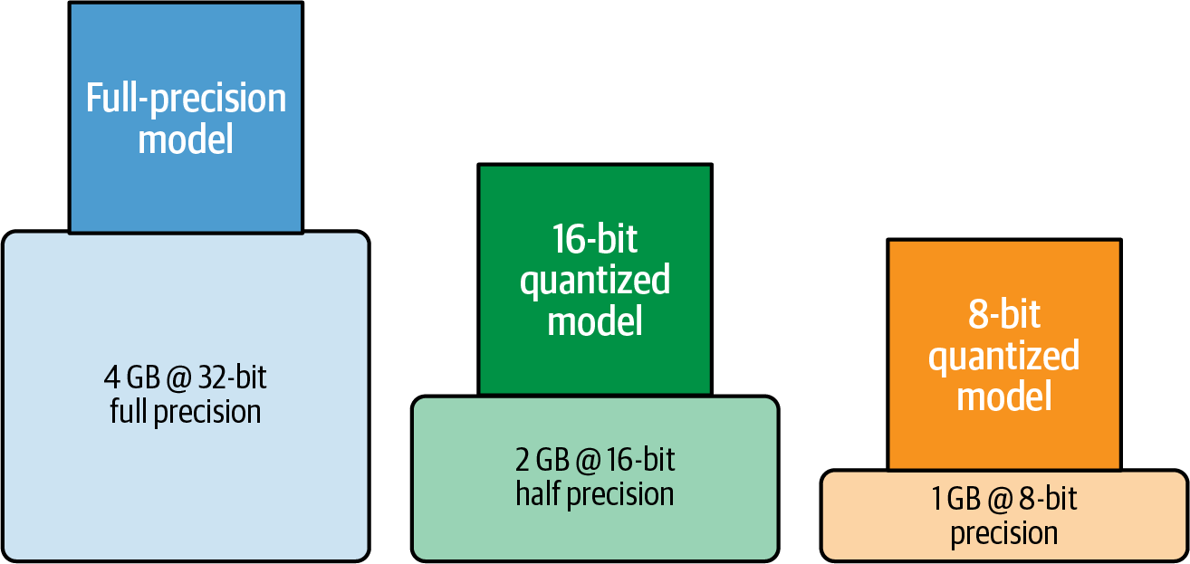
Figure 4-4. Approximate GPU RAM needed to load a 1-billion-parameter model at 32-bit, 16-bit, and 8-bit precision

Quantization projects a source set of higher-precision floating-point numbers into a lower-precision target set of numbers. Using the source and target ranges, the mechanism of quantization first calculates a scaling factor, makes the projection, then stores the results in reduced precision, which requires less memory and ultimately improves training performance and reduces cost.

fp16

With fp16, the 16 bits consist of 1 bit for the sign but only 5 bits for the exponent and 10 bits for the fraction, as shown in Table 4-3.

Table 4-3. fp32 versus fp16

	Sign	Exponent	Fraction (mantissa/significand)
fp32 (consumes 4 bytes of memory)	1 bit 0	8 bits 10000000	23 bits 10010010000111111011011
fp16 (consumes 2 bytes of memory)	1 bit 0	5 bits 10000	10 bits 1001001000

With the reduced number of bits for the exponent and fraction, the range of representable fp16 numbers is only from –65,504 to +65,504. You can also see this when you print the data type information for fp16:

torch.finfo(torch.float16)

The output is:

finfo(resolution=0.001, min=-65504, max=65504, eps=0.000976562, 
smallest_normal=6.10352e-05, tiny=6.10352e-05, dtype=float16)

Let’s store pi with 20 decimal places again in fp16 and compare the values:

pi = 3.14159265358979323846
pi_fp16 = torch.tensor(pi, dtype=torch.float16)
print('%.20f' % pi_fp16.item())

The output is:

3.14062500000000000000

Note the loss in precision after this projection, as there are only six places after the decimal point now. The fp16 value of pi is now 3.140625. Remember that you already lost precision just by storing the value in fp32, as shown in Figure 4-5.

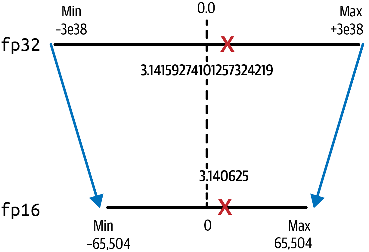
Figure 4-5. Quantization from fp32 to fp16 saves 50% memory

The loss in precision is acceptable in most cases, however. The benefits of a 50% reduction in GPU memory for fp16 compared to fp32 is typically worth the trade-off since fp16 only requires 2 bytes of memory versus 4 bytes of fp32.

Loading a 1-billion-parameter model now only requires 2 GB of GPU RAM, with 12 GB of GPU RAM needed for training the model, as shown in Figure 4-6.

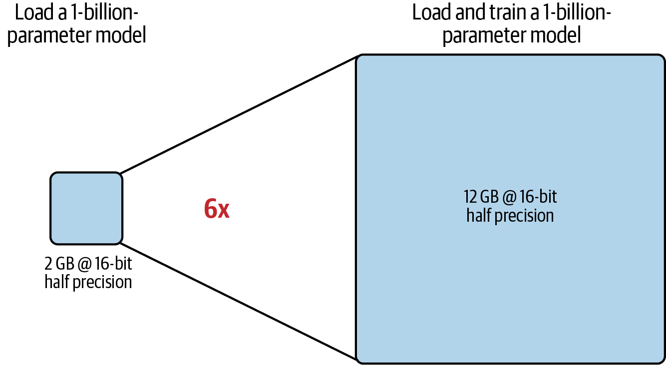
Figure 4-6. Only 12 GB of GPU RAM is needed to load and train a 1-billion-parameter model at 16-bit half precision

bfloat16

bfloat16 has become a popular alternative to fp16 as it captures the full range of fp32 with only 16-bits. This reduces numerical instabilities during model training caused by overflow. Overflow happens when numbers flow outside of the range of representation when converting them from a high-precision to a lower-precision space, causing NaN (not a number) errors.

Compared to fp16, bfloat16 has a greater dynamic range but less precision, which is usually acceptable. bfloat16 uses a single bit for the sign and the full 8 bits for the exponent. However, it truncates the fraction to just 7 bits, which is why it’s often called the “truncated 32-bit float,” as shown in Table 4-4.

Table 4-4. fp32 versus bfloat16

	Sign	Exponent	Fraction (mantissa/significand)
fp32 (consumes 4 bytes of memory)	1 bit 0	8 bits 10000000	23 bits 10010010000111111011011
bfloat16 (consumes 2 bytes of memory)	1 bit 0	8 bits 10000000	7 bits 1001001

The range of representable bfloat16 numbers is identical to fp32. Let’s print the data type information for bfloat16:

torch.finfo(torch.bfloat16)

The output is:

finfo(resolution=0.01, min=-3.38953e+38, max=3.38953e+38, eps=0.0078125, 
smallest_normal=1.17549e-38, tiny=1.17549e-38, dtype=bfloat16)

Let’s store pi with 20 decimal places again in bfloat16 and compare the values:

pi = 3.14159265358979323846
pi_bfloat16 = torch.tensor(pi, dtype=torch.bfloat16)
print('%.20f' % pi_bfloat16.item())

The output is:

3.14062500000000000000

Similar to fp16, bfloat16 comes with a minimal loss in precision. The bfloat16 value of pi is 3.140625. However, the benefits of maintaining the dynamic range of fp32 (shown in Figure 4-7) and thereby reducing overflow, usually outweighs the loss in precision.

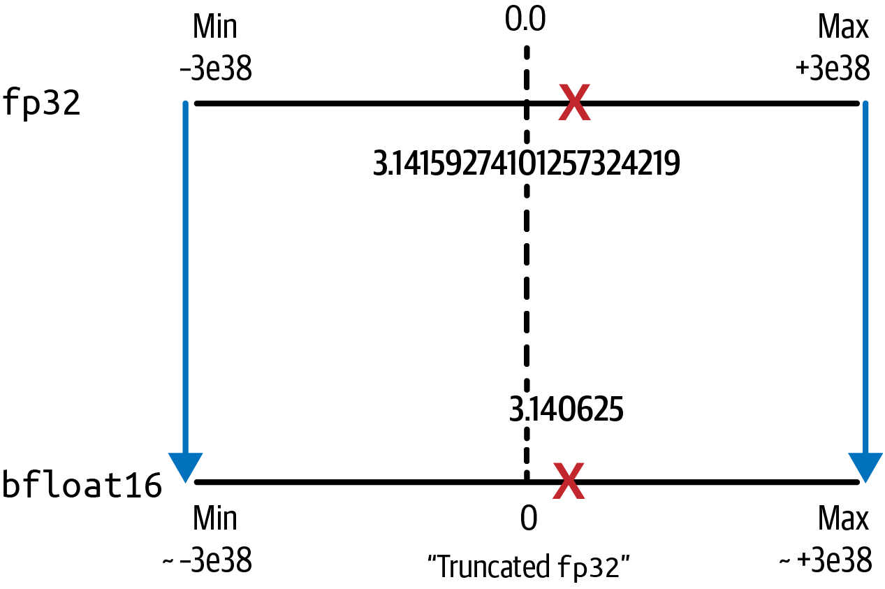
Figure 4-7. Quantization from fp32 to bfloat16 maintains the dynamic range of fp32 while still saving 50% memory

bfloat16 is natively supported by newer GPUs such as NVIDIA’s A100 and H100. Many modern generative AI models were pretrained with bfloat16, including FLAN-T5, Falcon, and Llama 2.

fp8

fp8 is a newer data type and natural progression from fp16 and bfloat16 to further reduce memory and compute footprint for multibillion-parameter models.

fp8 allows the user to configure the number of bits assigned to the exponent and fraction depending on the task, such as training, inference, or post-training quantization. NVIDIA GPUs started supporting fp8 with the H100 chip. AWS Trainium also supports fp8, called configurable fp8, or just cfp8. With cfp8, 1 bit is used for the sign, and the remaining 7 bits are configurable between the exponent and fraction, as shown in Table 4-5.

Table 4-5. fp32 versus fp8

	Sign	Exponent	Fraction (mantissa/significand)
fp32 (consumes 4 bytes of memory)	1 bit 0	8 bits 10000000	23 bits 10010010000111111011011
fp8 (consumes 1 byte memory)	1 bit 0	7 bits 0000011 (configurable)

Empirical results show that fp8 can match model training performance of fp16 and bfloat16 while reducing memory footprint by another 50% and speeding up model training.

int8

Another quantization option is int8 8-bit quantization. Using 1 bit for the sign, int8 values are represented by the remaining 7 bits, as shown in Table 4-6.

Table 4-6. fp32 versus int8

	Sign	Exponent	Fraction (mantissa/significand)
fp32 (consumes 4 bytes of memory)	1 bit 0	8 bits 10000000	23 bits 10010010000111111011011
int8 (consumes 1 byte of memory)	1 bit 0	n/a	7 bits 0000011

The range of representable int8 numbers is –128 to +127. Here’s the data type information for int8:

torch.iinfo(torch.int8)

The output is:

iinfo(min=-128, max=127, dtype=int8)

Let’s store pi with 20 decimal places again in int8 and see what happens:

pi = 3.14159265358979323846
pi_int8 = torch.tensor(pi, dtype=torch.int8)
print(pi_int8.item())

The output is:

3

Unsurprisingly, pi is projected to just 3 in the 8-bit lower precision space, as shown in Figure 4-8.

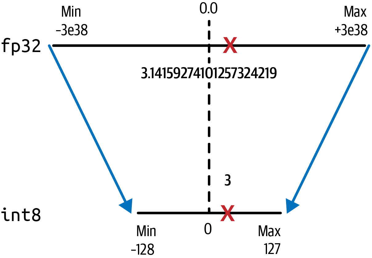
Figure 4-8. Quantization from fp32 to int8 saves 75% memory

This brings the memory requirement down from originally 4 bytes to just 1 byte, but results in a bigger loss of precision due to the conversion from a floating point representation to an integer value.

Reducing the memory footprint of large foundation models is not only helpful for loading and training models, but also for inference. Despite the loss in precision, 8-bit quantization is often used to improve inference throughput and latency for deployed models. Optimized implementations for int8 quantization such as Hugging Face’s bitsandbytes integration of LLM.int8(), have shown to minimize quantization impact on model performance. You will learn about post-training quantization (PTQ) and the technique GPT post-training quantization (GPTQ)¹ in more detail when you prepare the model for deployment in Chapter 8.

Table 4-7 compares the data types discussed thus far.

Table 4-7. Comparison of data types used for quantization

	Total bits	Sign bits	Exponent bits	Fraction bits	Memory needed to store one value
fp32	32	1	8	23	4 bytes
fp16	16	1	5	10	2 bytes
bf16	16	1	8	7	2 bytes
fp8	8	1	7		1 byte
int8	8	1	n/a	7	1 byte

In summary, the choice of data type for model quantization should be based on the specific needs of your application. While fp32 offers a safe choice if accuracy is paramount, you will likely hit hardware limits, such as available GPU RAM, especially for multibillion-parameter models.

In this case, quantization using fp16 and bfloat16 can help to reduce the required memory footprint by 50%. bfloat16 is usually preferred over fp16 as it maintains the same dynamic range as fp32 and reduces overflow. fp8 is an emerging data type to further reduce memory and compute requirements. Some hardware implementations allow configuring the bits for exponent and fraction; empirical results show performance can match model training with fp16 and bfloat16. int8 has become a popular choice to optimize your model for inference. fp8 is becoming more popular as both hardware and deep-learning framework support emerges.

Tip

It is recommended that you always benchmark the quantization results to ensure the selected data type meets your accuracy and performance requirements.

Another memory and compute optimization technique is FlashAttention. Flash­At⁠tention aims to reduce the quadratic compute and memory requirements, O(n²), of the self-attention layers in Transformer-based models.

Optimizing the Self-Attention Layers

As mentioned in Chapter 3, performance of the Transformer is often bottlenecked by the compute and memory complexity of the self-attention layers. Many performance improvements are targeted specifically at these layers. Next, you will learn some powerful techniques to reduce memory and increase performance of the self-attention layers.

FlashAttention

The Transformer’s attention layer is a bottleneck when trying to scale to longer input sequences because the computation and memory requirements scale quadratically O(n²) with the number of input tokens. FlashAttention, initially proposed in a research paper,² is a GPU-specific solution to this quadratic scaling problem.

FlashAttention, on version 2 as of this writing, reduces the amount of reads and writes between GPU main memory, called high-bandwidth memory (HBM), and the much faster but smaller on-chip GPU static RAM (SRAM). Despite its name, the GPU high-bandwidth memory is an order of magnitude slower than the on-chip GPU SRAM.

Overall, FlashAttention increases self-attention performance by 2–4x and reduces memory usage 10–20x by reducing the quadratic O(n²) computational and memory requirements down to linear O(n), where n is the number of input tokens in the sequence. With FlashAttention, the Transformer scales to handle much longer input sequences which allows for better performance on larger input context windows.

A popular implementation is installable with a simple pip install flash-attn --no-build-isolation command which installs the flash-attn library as a drop-in replacement for the original attention.

Attention optimizations are an active area of research, including the next generation FlashAttention-2,³ which continues to implement GPU-specific optimizations to improve performance and reduce memory requirements.

Let’s learn about another technique to improve the performance of the self-attention layers in the Transformer.

Grouped-Query Attention

Another popular optimization to the attention layers is grouped-query attention (GQA). GQA improves upon the Transformer’s traditional multiheaded attention, described in Chapter 3, by sharing a single key (k) and value (v) head for each group of query (q) heads (as opposed to each query head), as shown in Figure 4-9.

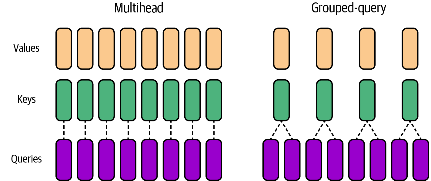
Figure 4-9. Grouped-query attention versus traditional multiheaded attention

GQA allows queries to be grouped into fewer key and value heads and therefore reduces memory consumption of the attention heads. In addition, GQA improves performance by reducing the number of memory reads and writes.

Since these improvements are proportional to the number of input tokens, MQA is particularly useful for longer input token sequences and allows for a larger context window. For example, the Llama 2 model by Meta uses GQA to improve performance and increase the input token context window size to 4,096—double the original LLaMA model’s 2,048 context window size.

Distributed Computing

For larger models, you will likely need to use a distributed cluster of GPUs to train these massive models across hundreds or thousands of GPUs. There are many different types of distributed computing patterns, including distributed data parallel (DDP) and fully sharded data parallel (FSDP). The main difference is how the model is split—or sharded—across the GPUs in the system.

If the model parameters can fit into a single GPU, then you would choose DDP to load a single copy of the model into each GPU. If the model is too large for a single GPU—even after quantization—then you need to use FSDP to shard the model across multiple GPUs. In both cases, the data is split into batches and spread across all available GPUs to increase GPU utilization and cost efficiency at the expense of some communication overhead, which you will see in a bit.

Distributed Data Parallel

PyTorch comes with an optimized implementation of DDP that automatically copies your model onto each GPU (assuming it fits into a single GPU using a technique such as quantization), splits the data into batches, and sends the batches to each GPU in parallel. With DDP, each batch of data is processed in parallel on each GPU, followed by a synchronization step where the results from each GPU (e.g., gradients) are combined (e.g., averaged). Subsequently, each model—one per GPU—is updated with the combined results and the process continues, as shown in Figure 4-10.

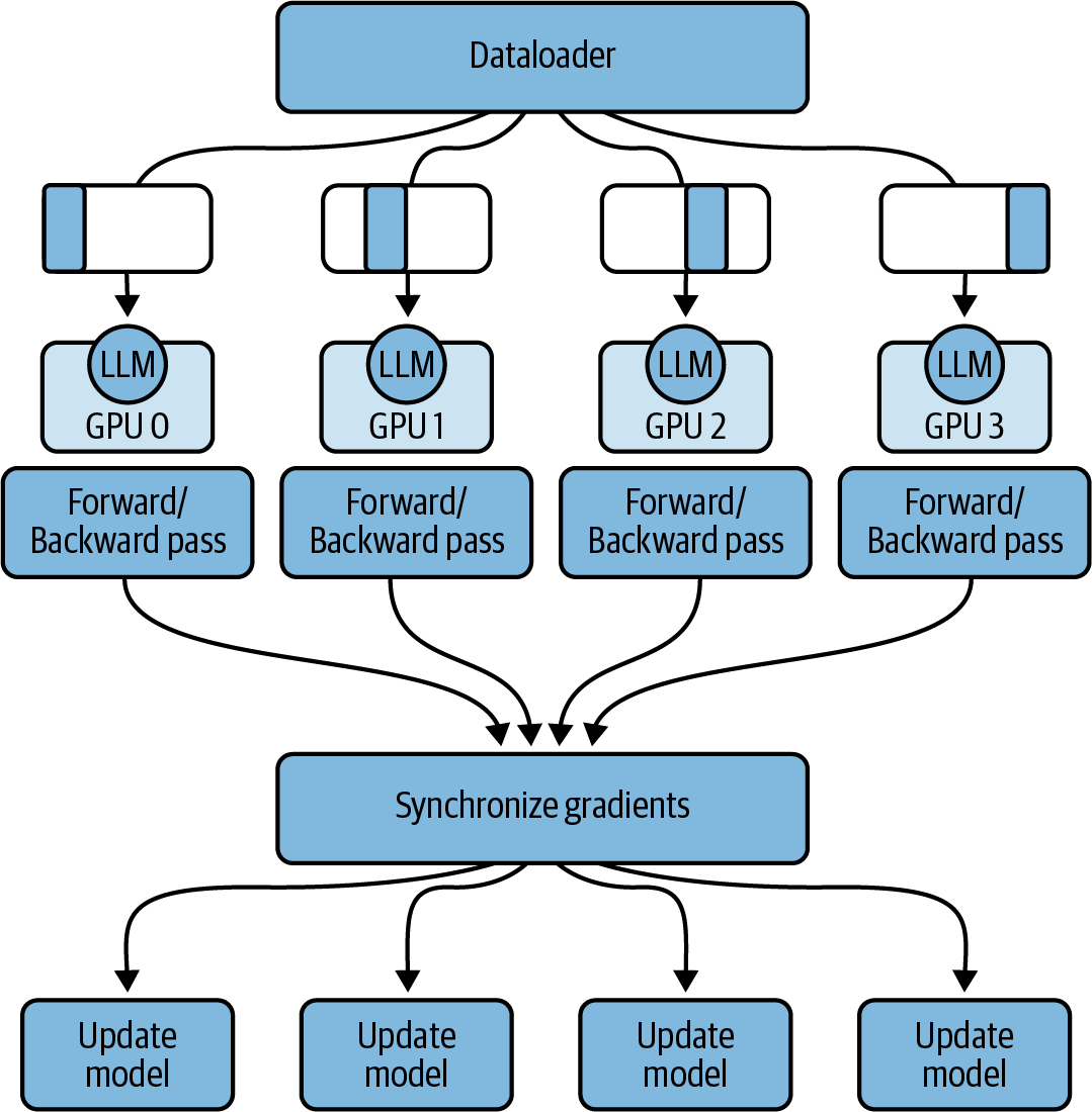
Figure 4-10. Distributed data parallel (DDP)

Note that DDP assumes that each GPU can fit not only your model parameters and data batches but also the additional data that is needed to fulfill the training loop, including optimizer states, activations, temporary function variables, etc., as shown in Figure 4-15. If your GPU cannot store all of this data, you need to shard your model across multiple GPUs. PyTorch has an optimized implementation of model sharding that you will see next.

Fully Sharded Data Parallel

FSDP was motivated by a 2019 ZeRO paper.⁴ The goal of ZeRO, or zero redundancy optimizer, is to reduce DDP’s data redundancy by sharding the model—and its additional gradients, activations, and optimizer states—across the GPUs to achieve zero redundancy in the system. ZeRO describes three optimization stages (1, 2, 3) depending on what is being sharded across the GPUs, as shown in Figure 4-11.

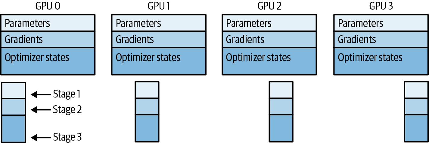
Figure 4-11. ZeRO consists of three stages depending on the GPU shards: parameters, gradients, and optimizer states

ZeRO Stage 1 only shards the optimizer states across GPUs but still reduces your model’s memory footprint up to 4x. ZeRO Stage 2 shards both the optimizer states and gradients across the GPUs to reduce GPU memory up to 8x. ZeRO Stage 3 shards everything—including the model parameters—across the GPUs to help reduce GPU memory up to n times, where n is the number of GPUs. For example, when using ZeRO Stage 3 with 128 GPUs, you can reduce your memory consumption by up to 128x.

Compared to DDP, in which each GPU has a full copy of everything needed to perform the forward and backward pass, FSDP needs to dynamically reconstruct a full layer from the sharded data onto each GPU before the forward and backward passes, as shown in Figure 4-12.

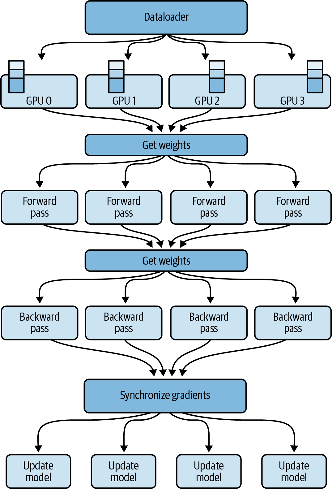
Figure 4-12. FSDP across multiple GPUs

In Figure 4-12, you see that before the forward pass, each GPU requests data from the other GPUs on-demand to materialize the sharded data into unsharded, local data for the duration of the operation—typically on a per-layer basis.

When the forward pass completes, FSDP releases the unsharded local data back to the other GPUs—reverting the data back to its original sharded state to free up GPU memory for the backward pass. After the backward pass, FSDP synchronizes the gradients across the GPUs, similar to DDP, and updates the model parameters across all the model shards, where different shards are stored on different GPUs.

By materializing the data on demand, FSDP balances the communication overhead with the overall GPU memory footprint. You can manually configure the sharding factor through the distributed computing configuration. Later in this chapter, you will see an example using Amazon SageMaker’s sharded_data_parallel_degree configuration parameter. This configuration setting helps to manage the trade-off between performance and memory utilization depending on your specific environment, as shown in Figure 4-13.

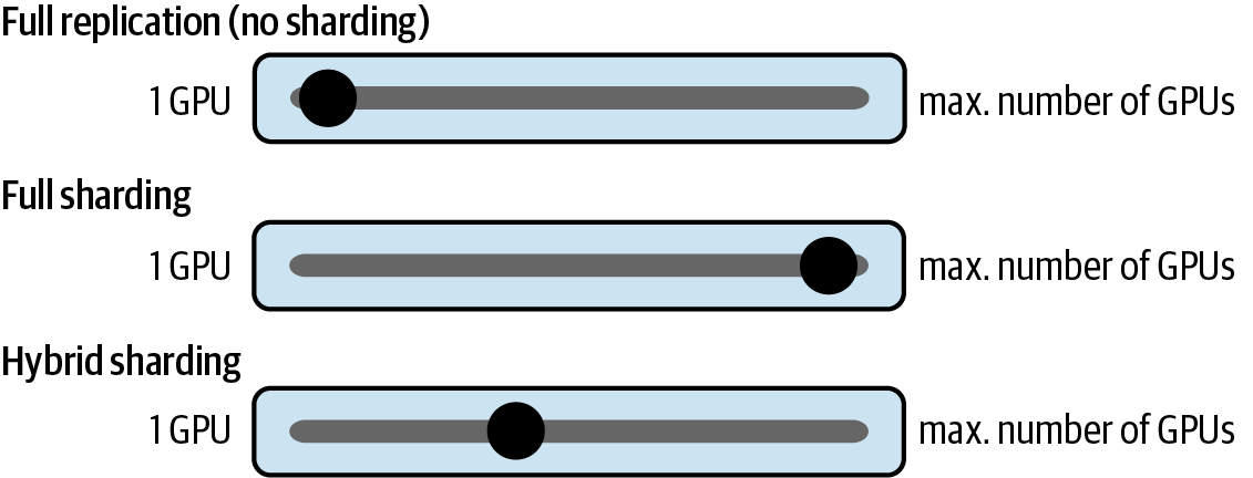
Figure 4-13. Choose a sharding factor based on the resources in your environment

A sharding factor of 1 avoids model sharding and replicates the model across all GPUs—reverting the system back to DDP. You can set the sharding factor to a maximum of n number of GPUs to unlock the potential of full sharding. Full sharding offers the best memory savings—at the cost of GPU-communication overhead. Setting the sharing factor to anything in between will enable hybrid sharding.

Performance Comparison of FSDP over DDP

Figure 4-14 is a comparison of FSDP and DDP from a 2023 PyTorch FSDP paper.⁵ These tests were performed on different-sized T5 models using 512 NVIDIA A100 GPUs—each with 80 GB of memory. They compare the number of FLOPs per GPU. A teraFLOP is 1 trillion floating point operations per second.

Figure 4-14. Performance improvement with FSDP over DDP (source: adapted from an image in Zhao et al.)

Note that full replication means there is no sharding. And since full replication is the equivalent of DDP, the performance of the full replication and DDP configurations are nearly identical.

For the smaller T5 models, 611 million parameters and 2.28 billion parameters, FSDP performs the same as DDP. However, at 11.3 billion parameters, DDP runs out of GPU memory, which is why there is no data for DDP in the 11.3 billion dimension. FSDP, however, easily supports the higher parameter size when using hybrid and full sharding.

Furthermore, training the 11-billion-parameter model with different cluster sizes from 8 GPUs to 512 GPUs shows only a 7% decrease in per-GPU teraFLOPs due to GPU communication overhead. These tests were run with batch sizes of 8 (blue) and 16 (orange), as shown in Figure 4-15, which is also sourced from the 2023 PyTorch FSDP paper.

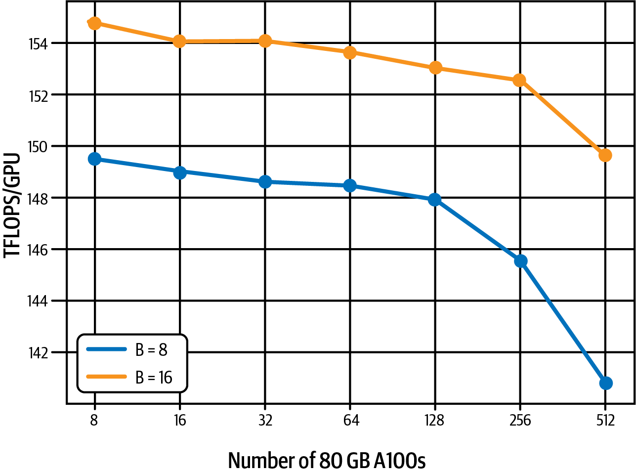
Figure 4-15. Only little performance decrease due to GPU communication overhead (source: adapted from an image in Zhao et al.)

This demonstrates that FSDP can scale model training for both small and large models across different GPU cluster sizes. Next, you will learn about performing distributed computing and FSDP on AWS using Amazon SageMaker.

Distributed Computing on AWS

Amazon SageMaker distributed training has been used to train some of the most powerful foundation models in the world, including Falcon and BloombergGPT. Falcon-180B, for example, was trained using an Amazon SageMaker distributed training cluster of 512 ml.p4d.24xlarge instances—each with 8 NVIDIA A100 GPUs (40 GB GPU RAM each) for a total of 4,096 GPUs and approximately 164 TB of GPU RAM. BloombergGPT was trained on 64 ml.p4d.24xlarge instances for a total of 512 GPUs and approximately 20TB of GPU RAM.

With SageMaker’s distributed computing infrastructure, you can run highly scalable and cost-effective generative AI workloads with just a few lines of code. Next, you will learn how to implement FSDP with Amazon SageMaker.

Fully Sharded Data Parallel with Amazon SageMaker

FSDP is a common distributed computing strategy supported by Amazon SageMaker. The following code shows how to launch an FSDP distributed training job using the PyTorch Estimator with 2 ml.p4d.24xlarge SageMaker instances—each with 8 GPUs and 320 GB of GPU RAM:

# Choose instance type and instance count 
# based on the GPU memory requirements 
# for the model variant we are using 
# e.g. Llama2 7, 13, 70 billion
instance_type = "ml.p4d.24xlarge" # 8 GPUs each
instance_count = 2 
# Set to the number of GPUs on that instance
processes_per_host = 8
# Configure the sharding factor
# In this case, 16 is the maximum, fully-sharded configuration
# since we have 2 instances * 8 GPUs per instance
sharding_degree = 16
# Set up the training job
smp_estimator = PyTorch(
  entry_point="train.py", # training script
  instance_type=instance_type,
  instance_count=instance_count,
  distribution={
      "smdistributed": {
          "modelparallel": {
              "enabled": True,
              "parameters": {
                  "ddp": True,
                  "sharded_data_parallel_degree":
                       sharding_degree
              }
          }
      },
      ...
  },
  ...
)

Here, configure the job to use smdistributed with modelparallel.enabled and ddp set to True. This configures the SageMaker cluster to use the FSDP distributed computing strategy. Note that we set the sharded_data_parallel_degree parameter to 16 because we have two instances with eight GPUs each. This parameter is our sharding factor, as discussed in the section “Fully Sharded Data Parallel”. Here, we choose full sharding by setting the value to the total number of GPUs in the cluster.

Next are some interesting snippets of the train.py referenced in the previous PyTorch Estimator code. The full code is in the GitHub repository associated with this book:

from transformers import AutoConfig, AutoModelForCausalLM
import smp # SageMaker distributed library

# Create FSDP config for SageMaker
smp_config = {
      "ddp": True,
      "bf16": args.bf16,
      "sharded_data_parallel_degree": args.sharded_data_parallel_degree,
}

# Initialize FSDP
smp.init(smp_config)

# Load HuggingFace model
model = AutoModelForCausalLM.from_pretrained(model_checkpoint)
# Wrap HuggingFace model in SageMaker DistributedModel class
model = smp.DistributedModel(
      model
)

# Define the distributed training step
@smp.step
def train_step(model, input_ids, attention_mask, args):
  if args.logits_output:
      output = model(input_ids=input_ids,
          attention_mask=attention_mask, 
          labels=input_ids)
      loss = output["loss"]
  else:
      loss = model(input_ids=input_ids, 
          attention_mask=attention_mask, 
          labels=input_ids)["loss"]
  model.backward(loss)
  if args.logits_output:
      return output

    return loss

Next, you will see how to train a model on AWS Trainium hardware, which is purpose-built for deep learning workloads. For this, you will learn about the AWS Neuron SDK—as well as the Hugging Face Optimum Neuron library which integrates the Hugging Face Transformers ecosystem with the Neuron SDK.

AWS Neuron SDK and AWS Trainium

The AWS Neuron SDK is the developer interface to AWS Trainium. Hugging Face’s Optimum Neuron library is the interface between the AWS Neuron SDK and the Transformers library. Here is an example that demonstrates the NeuronTrainer class from the Optimum Neuron library, which is a drop-in replacement for the Transformers Trainer class when training with AWS Trainium:

from transformers import TrainingArguments
from optimum.neuron import NeuronTrainer

def train():
    model = AutoModelForCausalLM.from_pretrained(
        model_checkpoint)

    training_args = TrainingArguments(
        ... 
    )

    trainer = NeuronTrainer(
        model=model,
        args=training_args,
        train_dataset=...,
        eval_dataset=...
    )

    trainer.train()

Summary

In this chapter, you explored computational challenges of training large foundation models due to GPU memory limitations and learned how to use quantization to save memory, reduce cost, and improve performance.

You also learned how to scale model training across multiple GPUs and nodes in a cluster using distributed training strategies such as distributed data parallel (DDP) and fully sharded data parallel (FSDP).

By combining quantization and distributed computing, you can train very large models efficiently and cost effectively with minimal impact on training throughput and model accuracy.

You also learned how to train models with the AWS Neuron SDK and AWS Trainium purpose-built hardware for generative deep learning workloads. You saw how to use the Hugging Face Optimum Neuron library, which integrates with the AWS Neuron SDK to improve the development experience when working with AWS Trainium.

In Chapter 5, you will learn how to adapt existing generative foundation models to your own datasets using a technique called fine-tuning. Fine-tuning an existing foundation model can be a less costly yet sufficient alternative to model pretraining from scratch.

¹ Elias Frantar et al., “GPTQ: Accurate Post-Training Quantization for Generative Pre-Trained Transformers”, arXiv, 2023.

² Tri Dao et al., “FlashAttention: Fast and Memory-Efficient Exact Attention with IO-Awareness”, arXiv, 2022.

³ Tri Dao, “FlashAttention-2: Faster Attention with Better Parallelism and Work Partitioning”, arXiv, 2023.

⁴ Samyam Rajbhandari et al., “ZeRO: Memory Optimizations Toward Training Trillion Parameter Models”, arXiv, 2020.

⁵ Yanli Zhao et al., “PyTorch FSDP: Experiences on Scaling Fully Sharded Data Parallel”, arXiv, 2023.