Excel Cookbook

Chapter 1. Workbooks, Worksheets, and Cells

Excel has many features and tools to help you save time and produce slick, polished spreadsheets.

This first chapter focuses on features generally useful when working with Excel files, such as themes and cell styles, defining templates, creating custom number formats, and using conditional formatting. It also covers time-saving tools such as Auto Fill, Flash Fill, and the Quick Access Toolbar and includes hidden gems such as custom lists and the Go To Special tool.

1.1 Using Themes

Problem

You have a workbook and want to apply a consistent look and feel to it.

Solution

When you create a new workbook, Excel applies a theme to it: a set of colors, fonts, and effects designed to give your workbook a consistent appearance. Excel includes several predefined themes, and you can switch to a different one by choosing Page Layout ⇒ Themes ⇒ Themes and selecting a theme from the Theme gallery.

You can also create a custom theme as follows:

1. Select a set of theme colors by choosing Page Layout ⇒ Themes ⇒ Colors and selecting a predefined color set. Alternatively, create a new custom color set by choosing Page Layout ⇒ Themes ⇒ Colors and selecting the Customize Colors option.

2. Select a set of fonts—a heading font and a body font—by choosing Page Layout ⇒ Themes ⇒ Fonts and selecting a predefined font set. Alternatively, create a new custom font set by choosing Page Layout ⇒ Themes ⇒ Fonts and selecting the Customize Fonts option.

3. Select a set of effects to change the appearance of any drawing objects by choosing Page Layout ⇒ Themes ⇒ Effects and selecting an effect; note that you can use only predefined effects and can’t create your own.

4. Save the colors, fonts, and effects as a theme by choosing Page Layout ⇒ Themes ⇒ Themes ⇒ Save Current Theme, and selecting a save location.

Once you’ve created a custom theme, apply it to a workbook by choosing Page Layout ⇒ Themes ⇒ Themes ⇒ Browse for Themes.

Discussion

A theme lets you apply a consistent look and feel to your workbook. You can choose one of Excel’s predefined themes or create a custom one to apply a corporate or personal style.

See Also

To change the default theme Excel applies to new workbooks, see Recipe 1.7.

1.2 Using Cell Styles

Problem

You’ve applied a theme to a workbook and want to use it to style selected cells.

Solution

You can apply a theme’s fonts and colors to cells using cell styles.

A cell style is a defined set of formatting characteristics—such as font, font size, and shading—that help you consistently style cells. Each style uses the fonts and colors associated with the workbook’s theme (see Recipe 1.1), so if you switch to a different theme, the cell styles update automatically.

To apply a cell style, select the cells you want to format, choose Home ⇒ Styles ⇒ Cell Styles, and select a style. The styles are grouped according to purpose as follows:

Good, Bad, and Neutral

These styles let you format cells containing particularly good or bad results.

Data and Model

These are for cells containing calculations, warnings, notes, or for cells that need input values.

Titles and Headings

This includes styles for different heading levels and a Total cell style.

Themed Cell Styles

These styles offer color accents based on the theme’s color palette.

Number Format

Use these styles to quickly format a number as a currency or percentage or to use commas as a thousands separator.

If you want to modify a cell style, you can do so by choosing Home ⇒ Styles ⇒ Cell Styles, right-clicking the style you want to modify, then choosing the Modify option from the shortcut menu. This opens the Style dialog box, which you can use to adjust the cell’s style with Excel’s cell formatting options (see Recipe 1.3).

To create a new style, you can either copy an existing style by right-clicking it and choosing the Duplicate option or create one from scratch by choosing Home ⇒ Styles ⇒ Cell Styles and clicking the New Cell Style option.

Tip

By default, custom styles are available only in the workbook in which you create them. You can, however, import styles from another open workbook by choosing Home ⇒ Styles ⇒ Cell Styles ⇒ Merge Styles.

Discussion

You can use this recipe with Recipe 1.1 to apply a consistent look and feel to a workbook’s cells.

1.3 Formatting Cells

Problem

You want to format one or more cells in a worksheet and want to know how.

Solution

Excel includes many options for modifying a cell’s format, such as changing the alignment or orientation of its contents, adding a border or background color, and adjusting the font. You can add these options to a cell style (see Recipe 1.2) or apply them to cells ad hoc.

Tip

It’s generally better to format cells using cell styles since these automatically update to fit your workbook’s theme.

You generally update the format using two main methods:

• Selecting the cell and using the available options in the Home menu.

• Using the Format Cells dialog box. You can open this by right-clicking the cells you want to format and selecting Format Cells, choosing Home ⇒ Cells ⇒ Format ⇒ Format Cells, or clicking the Format button in the Style dialog box (see Recipe 1.2).

Discussion

The Home menu and Format Cells dialog box offer convenient ways of modifying a cell or cell style’s appearance. Try experimenting with the available options.

1.4 Formatting a Cell’s Value

Problem

You want to change how a cell’s value is formatted using one of Excel’s predefined formats.

Solution

Suppose you have cells that contain numbers, dates, or times, and you want to change how they’re formatted. You can do so by applying a number format; for example, you can format numbers as percentages, fractions, or currency and change a date’s appearance to include a time component.

To change a cell’s number format, you select the cell—or cells—you want to format, open the Format Cells dialog box (see Recipe 1.3), and select a format from the Number tab. The available options include the following:

General

This is the default format Excel applies to most numbers so they appear how you type them. The format uses scientific (exponential) notation for large numbers with 12 or more digits, and if the cell isn’t wide enough, it rounds the numbers.

Number

This format is for general numbers. You can specify the number of decimal places to display, whether to use commas, and how to display negative numbers.

Currency and Accounting

These options format a number as a monetary value, where the Accounting format lines up the decimal points and currency symbols in a column, and the Currency format doesn’t. Excel uses the Currency format by default for any numbers you enter as a monetary value (for example, $14).

Date and Time

These provide date and time formats based on a locale. Excel uses these formats by default for any values it recognizes as a date or time.

Percentage

This option lets you specify a number as a percentage using a specified number of decimal places. Excel uses this format by default for any numbers you enter as a percentage, (for example, 12%).

Fraction

Use this option to format a number as a fraction. Excel uses this format by default for any numbers you enter as a fraction (for example, 1 1/2).

Scientific

This option formats numbers using scientific (exponential) notation, where you can specify the number of decimal places. Excel uses this format by default for any numbers you enter using scientific notation (for example, 1.23E+10).

Text

This treats the cell value as text, displaying it how it’s entered. You should use this option only for values you don’t want to use in calculations since it can lead to misleading results; if you type a number into a cell with a Text format, Excel may store the number as a text value, which number functions such as SUM interpret as 0.

Special

This lets you format a number as a zip code, phone number, or Social Security number, depending on the locale.

Custom

This option lets you apply a custom format (see Recipe 1.5).

Note

Changing a cell’s format modifies only its appearance, leaving its underlying value unchanged. To determine a cell’s actual value, select the cell and look in the formula bar, change the format to General, or choose Formulas ⇒ Formula Auditing ⇒ Show Formulas.

Discussion

This recipe offers an overview of Excel’s predefined number formats and what they’re for. Formatting numbers is generally a good idea since it makes them more consistent and easier to read.

1.5 Defining a Custom Number Format

Problem

You want to define your own format for numbers, dates, and times instead of using one of Excel’s predefined formats.

Solution

Suppose you have cells containing numbers, dates, or times and want to customize their appearance. You can do so by defining a custom number format.

You define a custom number format by opening the Format Cells dialog box (see Recipe 1.3), selecting the Number tab, choosing the Custom option, and typing the format in the Type box. You can either select and modify an existing format or create one from scratch.

Each custom number format has one to four code sections, each one separated by a semicolon. If you supply a single code section, Excel applies that format to all numbers, so the custom number format 0, for example, displays all numbers as integers. If you supply two code sections, Excel uses the first to format positive numbers and zeros and the second to format negative numbers. The custom number format 0.00;[Red]-0.00, for example, contains two code sections: the first formats positive numbers and zeros to two decimal places, and the second formats negative numbers to two decimal places, includes a minus sign, and makes the font color red. If you supply four code sections, Excel uses the sections to format positive numbers, negative numbers, zeros, and text, in that order.

You control how numbers are displayed using the following characters:

# (hash) and 0 (zero)

Use # to specify a number’s significant digits, so the custom number format #.## displays 1.678 as 1.68 and 0.6 as .6. Use 0 to include extra zeros, so the custom number format 0.## displays 0.678 as 0.68, and the format 000.00 displays 1.2 as 001.20.

? (question mark)

Use ? to specify significant digits and align numbers by the decimal point. So the custom number format 0.?? displays 123 as 123. and 1.678 as 1.68, lining up the decimal points.

, (comma)

Use a comma as a thousands separator to scale a number by a multiple of 1,000. So the custom number format #,##0.00 displays 1234 as 1,234.00, and the format 0, displays 1234 as 1.

% (percent)

Use % to display a number as a percentage, so the custom number format 0% displays 123 as 12300%.

_ (underscore)

Use an underscore followed by a character to display a space the same width as the character. The format _(0.00_);(0.00), for example, puts negative numbers in parentheses and adds a parenthesis-width space before and after any positive numbers so the numbers line up.

* (asterisk)

To repeat a character so that it fills the remaining width of the cell, prefix it with an asterisk, so the format *0# adds leading zeros.

Figure 1-1 shows some examples of using custom number formats to control how numbers are displayed.

Figure 1-1. Examples of using custom number formats

Note

Placeholders after a decimal point specify how many decimal places to round a number to. All digits to the left of the decimal point are displayed, irrespective of the number of placeholders.

You can also add extra characters to a number format. To add a text string, enclose it in double quotation marks and add it to the relevant code section. The format "Balance: "$0.00 prefixes a dollar amount with the text Balance:. The double quotes aren’t needed for many commonly used single characters, such as $, (, ), +, and -, so you can type these directly in the relevant code section. So the format 0.00;(0.00) puts any negative numbers in parentheses, and $0.00 includes a dollar symbol, positioned according to your system’s regional settings (see Figure 1-2).

Figure 1-2. Adding extra characters to custom number formats

If you want to display the default format for any code section, use General instead of a format code. For example, the custom format General;-General;0;General displays zeros as 0 and other values using the default format, prefixing negative numbers with a minus sign. You can also use the @ character as a placeholder for any entered text. See Figure 1-3 for some examples that use these format codes.

Figure 1-3. Examples of the General format and @

To change the font color for any code section, put the name of the color in square brackets and add it to the start of the section. The possible options are [Black], [Blue], [Cyan], [Green], [Magenta], [Red], [White], and [Yellow], so the format code [Green]0.00;[Red]-0.00;0;@ uses green for positive numbers, red for negative numbers, and the default color for zeros and text. You can also refer to a color by number using the syntax [ColorN], where N is a number from 1 to 56 that refers to one of the 56 colors in the standard color palette. For example, [Color10] refers to a different shade of green than using [Green].

If you want to change the color of values subject to some condition, put the condition in a separate set of square brackets. The format [Red][<100]#0;[Blue][>=100]#0 changes the font color to red for numbers less than 100 and blue for numbers greater than or equal to 100. Similarly, the format [Red][<100]#0;[Blue][>1000]#0;#0 changes the font color to red for numbers less than 100, blue for numbers greater than 1,000, and uses the default font color for all other numbers.

Note

You can specify only up to two conditions in a custom number format. See Recipe 1.9 for a more flexible alternative.

You can also use custom number formats to format dates and times since, behind the scenes, dates and times are stored as numbers (see “Discussion”). You format the different components of a date/time value as follows:

Years

Use yy to format the year using two digits and yyyy to format it using four digits.

Months

Use m to format the month using one or two digits (1 to 12), mm to format it as two digits (01 to 12), mmm to display its short name (Jan to Dec), mmmm to display its full name (January to December), and mmmmm to display its initials (J to D).

Days

Use d to format the day using one or two digits (1 to 31), dd to format it using two digits (01 to 31), ddd to display the short name of its weekday (Sun to Sat), and dddd to display the full name (Sunday to Saturday).

Hours

Use h to format the hours using one or two digits (0 to 23) and hh to display two digits (00 to 23). By default, hours are based on a 24-hour clock; use AM/PM to use a 12-hour clock instead.

Minutes

Use m to format the minutes using one or two digits (0 to 59) and mm to display two digits (00 to 59).

Seconds

Use s to format the seconds using one or two digits (0 to 59) and ss to display two digits (00 to 59). You can also include hundredths of a second using ss.00.

Elapsed time

You can display elapsed time by putting the relevant time component in square brackets. The format [h]:mm shows the elapsed time in hours and minutes, while [mm]:ss shows it in minutes and seconds.

See Figure 1-4 for examples of using date and time format codes.

Figure 1-4. Using custom number formats to control how dates and times are displayed

Discussion

This recipe describes how to define a custom number format, which is handy if none of Excel’s predefined formats (see Recipe 1.4) display cell values how you want.

Tip

You can skip sections using semicolons (;) to hide any values in that section. The format 0;-0;;@, for example, hides zeros, while using ;;; hides all values.

1.6 Merging Cells

Problem

You want to create a larger cell by merging several cells.

Solution

Suppose you want to make a cell larger by making it span more than one row and/or column. You can do so by merging cells as follows:

1. Select the cells you want to merge.

2. Choose Home ⇒ Alignment ⇒ Merge & Center to merge the cells into one and center its contents. Alternatively, open the Merge & Center drop-down menu and select Merge Cells to merge the cells without centering the contents or Merge Across to merge the selected cells in rows.

To unmerge cells, choose Home ⇒ Alignment, open the Merge & Center command’s drop-down menu, and select Unmerge.

Discussion

This recipe shows how to create a larger cell spanning multiple rows and/or columns; this can be handy if, for example, you want to insert text or a formula that’s relevant to multiple rows. It’s also handy if you want to increase the size of a sparkline; see Recipe 13.10.

1.7 Creating Templates

Problem

You want to be able to quickly create a workbook that uses a specified theme or contains prefilled cells.

Solution

Suppose you want Excel to automatically apply a specific theme to each new workbook you create, or you want to prefill new workbooks with the same layout, formatting, and formulas. In these situations, you can use a template: a partially completed workbook as a starting point for other workbooks.

Before creating the template, you must first set or find the location of the default personal templates folder. How you do this depends on whether you’re using Excel for Windows or Mac.

If you’re using Windows, follow these steps (see Figure 1-5):

1. In Excel, choose File ⇒ Options ⇒ Save.

2. Make a note of the folder in the Default personal templates location box, which is in the Save Workbooks section. If this box is empty, you’ll need to type the location yourself; this is typically c:\Users\<UserName>\Documents\Custom Office Templates, where <UserName> is your Windows username.

3. Click OK if you’ve made any changes, or Cancel if you haven’t.

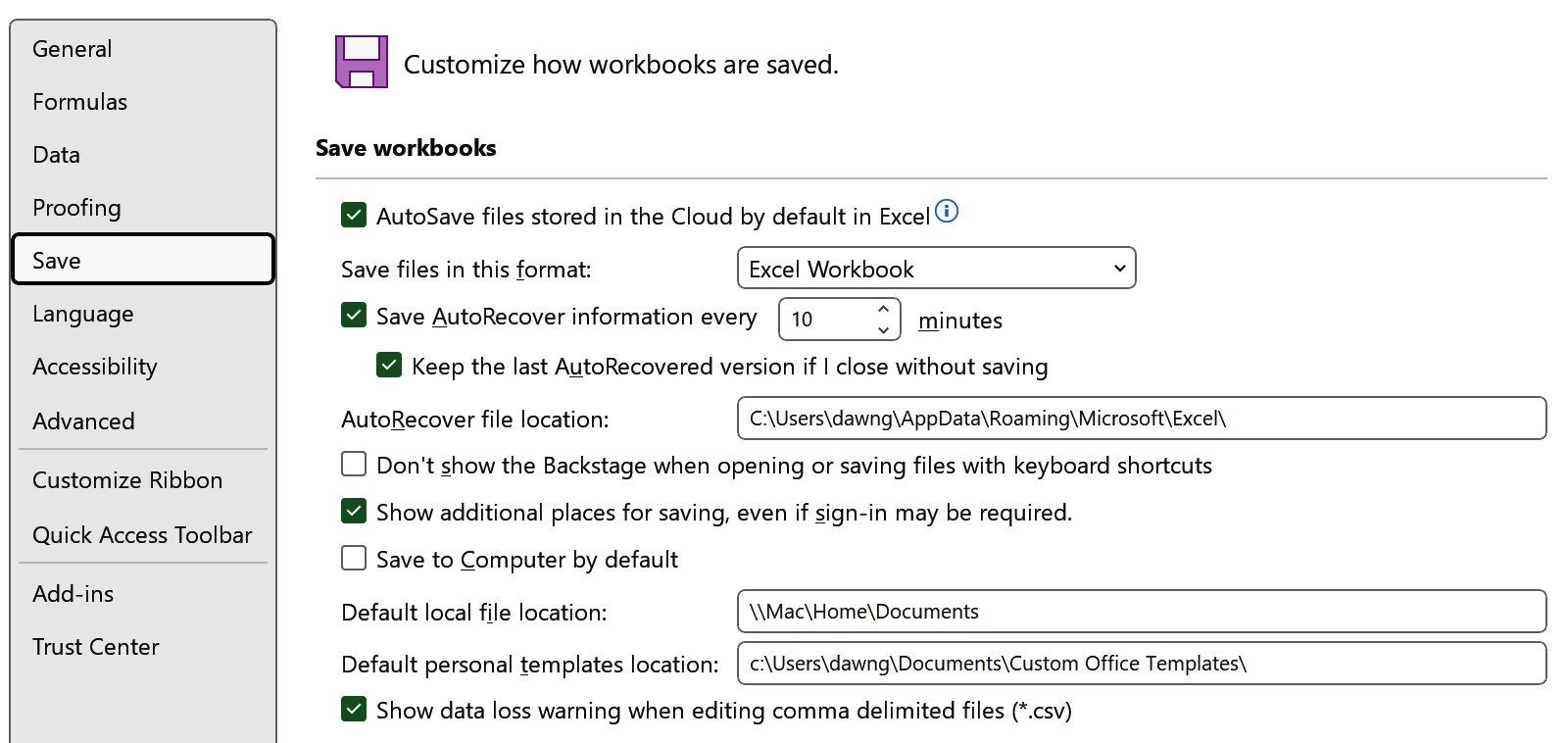
Figure 1-5. The Windows Default personal templates location box is toward the end of the Save Workbooks section

If you’re using Excel for Mac:

1. Open Word¹ and choose Word ⇒ Preferences ⇒ File Locations.

2. Make a note of the folder in the User templates box; this is typically /Users/<UserName>/Library/Group Containers/UBF8T346G9.Office/User Content/Templates, where <UserName> is your username.

3. Close the File Locations dialog box.

Once you’ve made a note of the default personal templates folder, you can create the template as follows:

1. Create an Excel workbook that includes everything you want to appear in the template. For example, you may want to apply a custom theme or prefill some of the cells with formulas.

2. Choose File ⇒ Save As if you’re using Excel for Windows, or File ⇒ Save as Template if you’re using Excel for Mac. Browse to the default personal templates folder and change the Save As Type to Excel Template—or Excel Macro-Enabled Template if the file contains macros (see Chapter 18).

3. Click Save to save the template; then close the file.

To create a new workbook based on the template, choose File ⇒ New and select your template from the Personal section.

Discussion

Custom templates offer a handy way of prefilling cells in a new workbook or automatically applying a default theme. They’re helpful in situations where, for example, you make a copy of an older workbook and edit the parts you need to change.

This recipe describes how to create a workbook template. To create a chart template, see Recipe 12.22.

1.8 Protecting Excel Files, Workbooks, Worksheets, and Cells

Problem

You want to protect a workbook and need to know Excel’s available options.

Solution

Excel includes various features to help protect your work from accidental changes, depending on what you want to achieve and your version of Excel.

To add passwords that control whether users have read-only access to an Excel file or can modify it, use file-level protection. To find these options, open the workbook and choose File ⇒ Info ⇒ Protect Workbook in Excel for Windows, or use the options in the File menu in Excel for Mac.

Warning

Using a password to protect your work doesn’t guarantee 100% security, especially when using older versions of Excel. Be careful when sharing files and passwords with others, and consider storing your files in a secure location.

Use workbook-level protection to control what users can do inside a workbook’s structure, such as adding or deleting worksheets. You can enable this option by choosing Review ⇒ Protect ⇒ Protect Workbook.

To control what users can do in a worksheet, use worksheet-level protection. You can enable this option by choosing Review ⇒ Protect ⇒ Protect Sheet or by right-clicking the worksheet’s tab and choosing Protect Sheet.

To protect a cell, apply a cell style (see Recipe 1.2) or format that includes protection. Set protection at this level by opening the Format Cells dialog box (see Recipe 1.3) and using the options on the Protection tab to lock or hide the cell.

Tip

You can hide rows, columns, and worksheets by right-clicking them and selecting Hide. Alternatively, select the rows, columns, or worksheets you want to hide and choose Home ⇒ Cells ⇒ Format ⇒ Hide & Unhide.

Discussion

This recipe offers a helpful overview of Excel’s built-in protection features, which you can use to prevent users from accidentally changing your work.

1.9 Using Conditional Formatting

Problem

You want to format one or more cells differently based on their contents.

Solution

Conditional formatting lets you format a cell range based on each cell’s contents. You can use it to identify large, small, or intermediate values, for example, or highlight cells that meet a certain set of rules that you specify.

To apply conditional formatting, select the range you want to format and choose Home ⇒ Styles ⇒ Conditional Formatting, and select one of the following options (see Figure 1-6):

Highlight Cells Rules

This option lets you apply a format (see Recipe 1.3) to cells whose values are within a specific numeric range, contain a given text string, are within a specific date range relative to today’s date, or that contain duplicate or unique values.

Top/Bottom Rules

This lets you apply a format to the top or bottom 10 or 10% values or ones above or below the range’s average value.

Data Bars

This adds data bars proportional to each cell’s value to help identify relatively large, small, or intermediate values.

Color Scales

This adds shading to each cell that’s proportional to each cell’s value. Similarly to data bars, this option helps you identify relatively large, small, or intermediate values.

Icon Sets

This adds an icon to each cell based on its value. As with data bars and color scales, this option helps you identify relatively large, small, or intermediate values.

New Rule

This option lets you define other conditional formatting rules, such as when a formula evaluates to TRUE (see Recipes 2.2 and 7.5); you can also define new rules by choosing one of the previous options and selecting More Rules.

Figure 1-6. Examples of using conditional formatting

The Conditional Formatting menu also includes a Clear Rules option, which lets you remove conditional formatting from the selected cells, a table, a PivotTable, or the worksheet, and a Manage Rules option, which opens the Conditional Formatting Rules Manager. The Rules Manager provides an overview of the rules in particular worksheets, tables, or selected cells, and lets you create new conditional formatting rules; view, edit, delete, and duplicate any existing ones; and update which cells they apply to (see Figure 1-7).

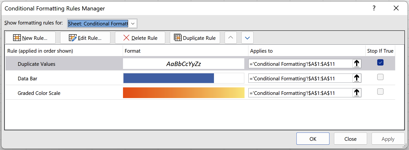
Figure 1-7. The Conditional Formatting Rules Manager

The Rules Manager lists rules in priority order, where the highest-priority rule is at the top and the lowest-priority rule is at the bottom. Excel applies rules in priority order, from the lowest rule upward, so if two rules conflict—for example, they apply different color scales to the same cells—Excel applies the rule with the highest priority that’s highest in the list. You can change a rule’s priority by selecting it and clicking the up or down arrows in the Rules Manager.

The Rules Manager also displays a Stop If True check box next to each rule. This check box controls whether lower-priority rules should run; once checked, it stops any lower-priority rules from being applied to cells where the checked rule is true.

Discussion

Applying conditional formatting offers a handy way of visualizing numeric data or highlighting cells whose values meet some condition. You can either use Excel’s predefined rules or create your own.

See Recipe 2.2 for more details about using conditional formatting with formulas.

1.10 Using the Format Painter

Problem

You want to quickly apply one cell’s format to another cell or range.

Solution

Excel’s Format Painter lets you copy a cell’s format and apply it to another cell or range. You use it as follows:

1. Select the cell whose format you want to copy.

2. Choose Home ⇒ Clipboard ⇒ Format Painter—the button with a paintbrush image.

3. Select the cells you want to apply the format to.

4. When you release the mouse button, Excel applies the original cell’s format.

Tip

To apply the format to multiple locations, double-click the Format Painter button. The Format Painter remains active until you select the Format Painter again or press the Esc key.

Discussion

This recipe offers a quick, convenient way of copying a cell’s format to one or more locations. Note that if you want to copy a cell’s contents in addition to its format, Recipe 1.11 may be more efficient.

1.11 Using Paste Special

Problem

You want to copy and paste a cell’s or range’s contents and/or attributes or use it to perform arithmetic operations on another range.

Solution

Excel’s Paste Special tool lets you copy a cell or range and select which contents or attributes—such as the values calculated by a formula or selected formatting—to paste elsewhere. You can also use this tool to transpose rows and columns, add the copied values to another set of values, or subtract, multiply, or divide by them.

To use Paste Special, follow these steps (see Figure 1-8):

1. Select the cells you want to copy.

2. Copy the cells by pressing Ctrl+C or choosing Home ⇒ Clipboard ⇒ Copy.

3. Select the first cell of the area you want to paste values to.

4. Select Home ⇒ Clipboard, open the Paste button’s menu, and choose Paste Special to open the Paste Special dialog box.

5. Select the options you want to use and click OK.

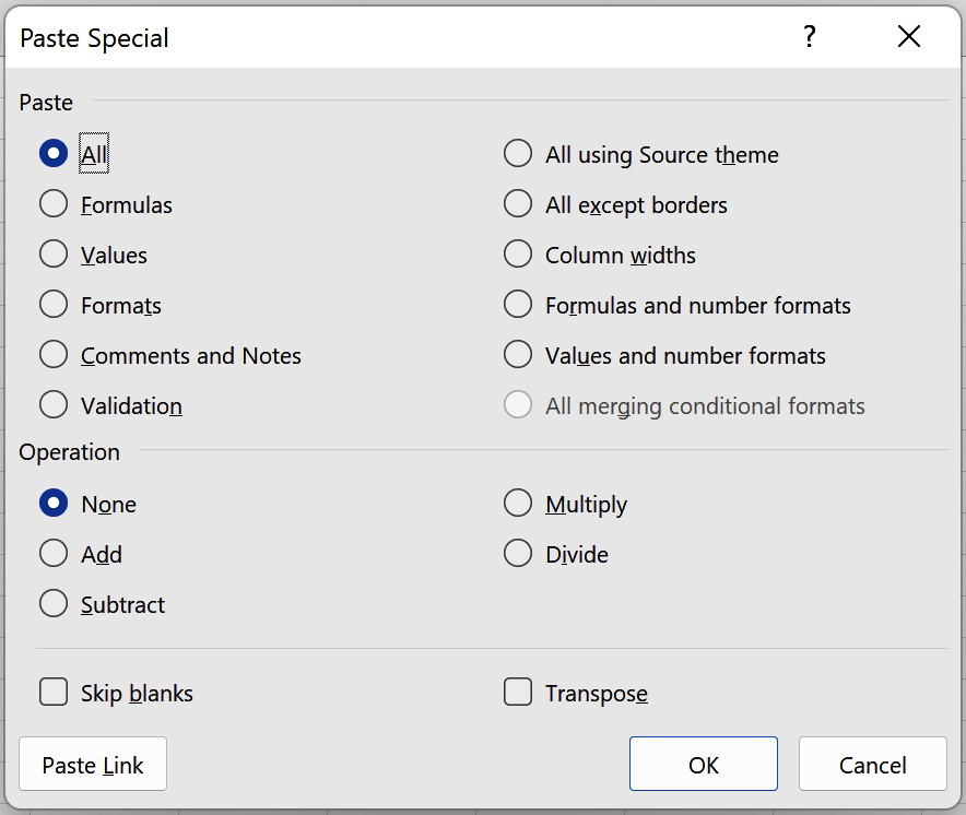
Figure 1-8. The Paste Special dialog box

Discussion

Paste Special offers a convenient way of copying one or more cells, pasting their contents and/or attributes to another location, and transposing cells. Note that if you want to only copy a cell’s format, you may find Recipe 1.10 more efficient.

1.12 Using Auto Fill

Problem

You want to fill cells with data that follows a series or pattern based on the contents of other cells.

Solution

Suppose you want to fill a cell range with a sequence of values, such as the numbers 1 to 10, or the weekdays from April 8, 2024 to May 6, 2024. You can do so using Excel’s Auto Fill tool.

Auto Fill helps you quickly fill cells based on the contents of other cells. You can use it, for example, to complete a series that increases in regular steps, copy a repeating pattern, complete a growth trend, or copy a formula to a range of cells. You generally use Auto Fill as follows:

1. Enter the first one or two values in the first cells of the range you want to fill. To fill the range A1:A10 with the numbers 1 to 10, for example, you’d type 1 in cell A1 and 2 in cell A2.

2. Select the cells you’ve just entered values into, click the selection’s square fill handle in its bottom-right corner, and drag it across the cells you want to fill. When you release the mouse button, Excel fills the cells.

Tip

If Auto Fill doesn’t work, you can enable it in Excel for Windows by choosing File ⇒ Options ⇒ Advanced and checking the Enable fill handle check box in the Editing options section. You can find this option in Excel for Mac by choosing Excel ⇒ Preferences ⇒ Edit.

You can adjust the Auto Fill tool’s output by clicking the Auto Fill Options button Excel displays next to the filled cells (see Figure 1-9) and selecting one of the options from its menu. So instead of filling the cells with a sequence, you can copy the original cells to create a repeating pattern, copy only the cell formatting, complete the series without including any formatting, or use Flash Fill (see Recipe 1.14). If the cells contain dates, you can also fill the series using days, weekdays, months, or years (see Figure 1-9).

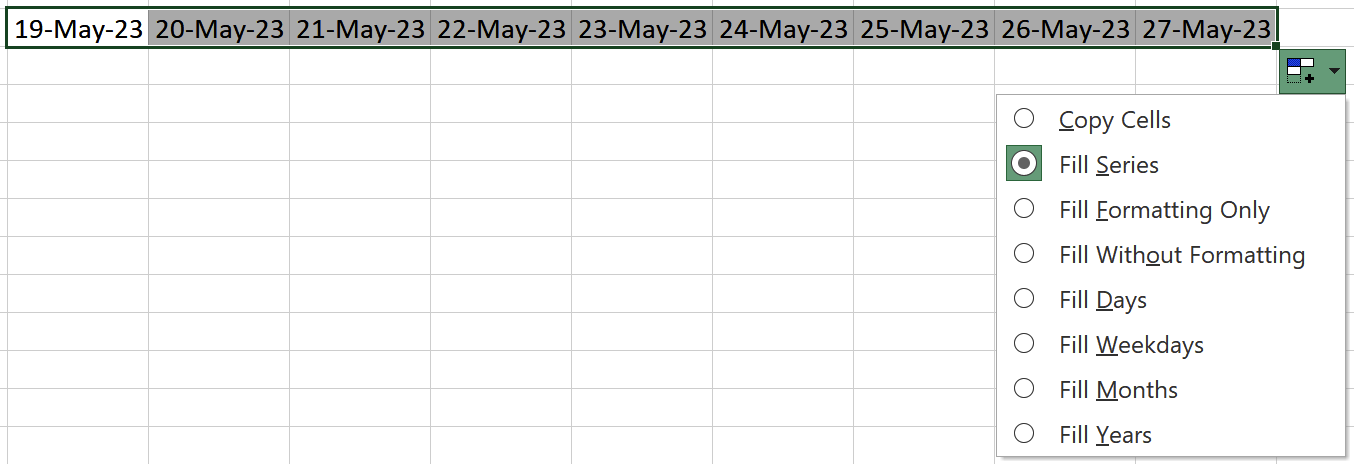
Figure 1-9. The Auto Fill Options menu

Tip

If the Auto Fill Options button doesn’t appear, you can enable it in Excel for Windows by choosing File ⇒ Options ⇒ Advanced and checking the Show Paste Options check box in the “Cut, copy, and paste” section. You can find this option in Excel for Mac by choosing Excel ⇒ Preferences ⇒ Edit.

If there are values next to the column or row you need to fill, you can double-click the fill handle in step 2 instead of dragging it, and Excel will deduce how many cells it needs to fill. This facility is handy if, for example, you need to fill an extensive range with sequential values.

If you want to fill the cells with a linear or growth trend or make further adjustments to the fill series, you can do so by right-clicking and dragging the fill handle in step 2 instead of clicking it. Doing so opens a menu containing extra Linear, Growth, and Series options; selecting the Series option opens the Series dialog box shown in Figure 1-10, which you can use to fine-tune how you want to fill cells.

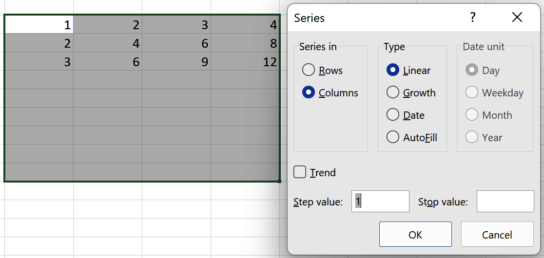
Figure 1-10. The Series dialog box

Discussion

Auto Fill is one of Excel’s most flexible tools because you can use it to copy values, formulas, attributes, and continue series. You can even use it to populate cells from a custom list (see Recipe 1.13). This recipe gives an overview of its many features, including those less well-known.

1.13 Using Custom Lists

Problem

You want to create a custom list of text values to populate cells with Auto Fill or use the list to sort values.

Solution

Suppose you frequently need to populate a cell range with a list of text values—for example, the values North, South, East, and West—and you want to be able to do this using Auto Fill. You additionally want to be able to sort these values in a specific order.

You can achieve this by defining a custom list: an ordered list of text values stored on your computer. To define a custom list (see Figure 1-11):

1. If you’re using Excel for Windows, choose File ⇒ Options ⇒ Advanced and click the Edit Custom Lists option in the General section to open the Custom Lists dialog box. If you’re using Excel for Mac, choose Excel ⇒ Preferences ⇒ Custom Lists instead.

2. Select NEW LIST from the Custom Lists section, click in the List Entries box, and type the orders you want to appear in the list using the Enter/Return key to separate entries. To define a custom list containing the values North, South, East, and West, for example, you’d type North in the List Entries box, press Enter/Return, then type South, and so on.

3. When you’ve finished typing all the entries, click the Add button to add the list to your system. Then click the OK button to close the dialog box.

Tip

You can also define a custom list by importing values from a cell range. Instead of typing the entries in the List Entries box in step 2, add the cell range to the Import list from cells box in the Custom Lists dialog box and click the Import button.

Once you’ve created the custom list, you can use it to populate cells using Auto Fill. So if you’ve defined a custom list containing North, South, East, and West, for example, you can populate the range A1:A4 with these values by typing North in A1, South in A2, and then using Auto Fill to populate A3 and A4 with the values East and West (see Recipe 1.12).

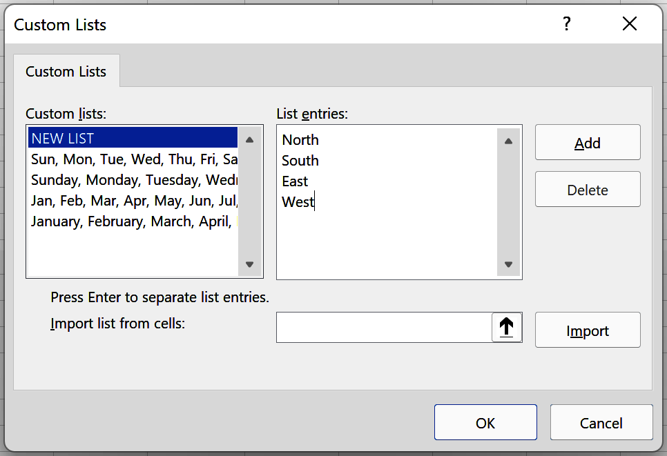
Figure 1-11. The Custom Lists dialog box

If you want to edit or delete a custom list, select it in the Custom Lists dialog box, edit its entries, or click the Delete button. Note that you can’t edit or delete any of Excel’s built-in lists, such as days of the week and months of the year.

Discussion

Custom lists can be helpful if you regularly want to Auto Fill cell ranges with the same list of text values. You can also use them to sort data in a specific order.

1.14 Using Flash Fill

Problem

You need to extract or concatenate data and want Excel to fill the remaining cells when it spots a pattern.

Solution

Suppose cells A2:A10 list customer first names and last names, and you want to extract the customer first names to cells B2:B10 (see Figure 1-12). You can do so using Flash Fill: a tool that analyzes the date you’re entering and uses pattern recognition to fill the remaining cells.

To use Flash Fill, you first enter a few examples of the results you want in a column next to the data. If you’re using Excel for Windows, it automatically launches Flash Fill when it spots a pattern and shows you a preview of the data it will fill, which you can accept by pressing Enter/Return. If you start typing the customer first names in cells B2 and B3, for example, Excel quickly recognizes what you’re doing and starts Flash Fill (see Figure 1-12).

Figure 1-12. Customer names and the Flash Fill preview

Tip

If you’re using Excel for Windows and Flash Fill doesn’t start automatically, you may need to enable this facility by choosing File ⇒ Options ⇒ Advanced and checking the Automatically Flash Fill check box in the Editing options section.

If you’re using Excel for Mac or you want to start Flash Fill manually, enter a few examples of the results you want, and then choose Data ⇒ Data Tools ⇒ Flash Fill or select Flash Fill from the Auto Fill Options menu (see Recipe 1.12).

Once you’ve accepted a Flash Fill preview, Excel displays a Flash Fill Options button next to the filled cells. When you click this button, Excel displays a menu that lets you undo the Flash Fill, accept the suggestions, select any blank cells, or select the cells that the Flash Fill completed (see Figure 1-13).

Tip

If you want to extract numeric codes—for example, telephone numbers or zip codes—you can get Flash Fill to include any leading zeros and numeric symbols by prefixing the text you type with an apostrophe. The apostrophe tells Excel to treat the codes as text, so typing '+44 is interpreted as the text +44, while typing +44 is interpreted as the positive number 44 without a leading plus sign.

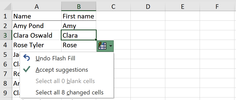
Figure 1-13. The Flash Fill Options menu

Discussion

Flash Fill offers a fast and simple solution when you want to extract or concatenate data. Note that data populated using Flash Fill isn’t dynamically updated, so if the underlying data changes, you’ll need to update the filled text or use Flash Fill again. Alternatively, use the recipes in Chapter 5 to create a more dynamic, formula-based solution.

Note

If you have one or more cells containing text separated by a delimiter—for example, a comma—you can split it into columns using the Text to Columns Wizard. To access this tool, select the cells you want to split and choose Data ⇒ Data Tools ⇒ Text to Columns.

1.15 Customizing AutoCorrect

Problem

You want Excel to change abbreviations to full text, longer phrases, or symbols automatically.

Solution

Suppose that each time you type a short code in a cell, you want Excel to replace it with longer text. You can do so by adding the code and text to Excel’s AutoCorrect options (see Figure 1-14):

1. If you’re using Excel for Windows, choose File ⇒ Options ⇒ Proofing and click AutoCorrect Options to open the AutoCorrect dialog box. If you’re using Excel for Mac, choose Excel ⇒ Preferences ⇒ AutoCorrect.

2. Enter the code and the text you want to replace it with in the Replace and With boxes; then click Add.

3. Update any other options you want; then click OK to close the dialog box.

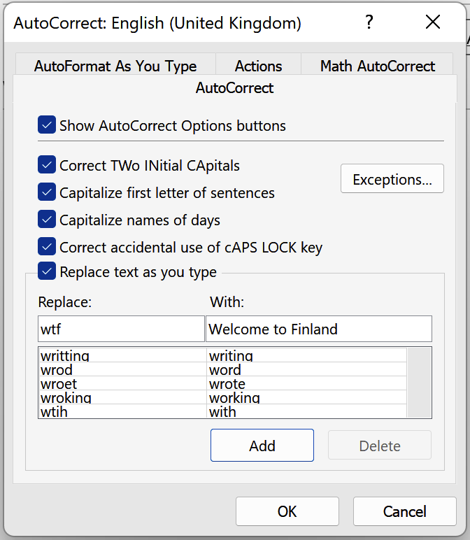
Figure 1-14. The AutoCorrect dialog box

Tip

If you want to replace a code with a symbol, first choose Insert ⇒ Symbols ⇒ Symbol, search for the symbol you wish to use, then copy it by pressing Ctrl+C. You can then paste the symbol in the AutoCorrect dialog box’s With box by pressing Ctrl+V.

Discussion

This recipe is a handy, time-saving technique for entering the same phrase or symbol many times.

1.16 Using Notes and Comments

Problem

You want to annotate a cell with a note or add a comment others can reply to.

Solution

If you’re using Excel 365, you can annotate cells using comments and notes. A comment is a threaded annotation that includes a Reply box, while a note is an unthreaded annotation without a Reply box (see Figure 1-15).

Figure 1-15. Notes versus comments

Note

Before Excel 365, Excel included only comments, not notes. The old version of comments worked similarly to notes in Excel 365.

To add a comment to a cell, select the cell and choose Review ⇒ Comments ⇒ New Comment, or right-click the cell and choose New Comment. Then type a comment in the Reply or Start a Conversation box and post it. Excel displays the comment when you hover your mouse cursor over the cell, and you can view and manage all the comments in a workbook by choosing Review ⇒ Comments ⇒ Show Comments, which opens Excel’s Comments pane.

To add a note, select the cell and choose Review ⇒ Notes ⇒ New Note, or right-click the cell and choose New Note. You then type the text you want to appear in the note. Excel displays the note when you hover your mouse cursor over the cell, select the cell and choose Review ⇒ Notes ⇒ Show/Hide Note, or right-click the cell and select Show/Hide Note. You can see all notes by choosing Review ⇒ Notes ⇒ Show All Notes, and you can convert notes to comments by choosing Review ⇒ Notes ⇒ Convert to Comments.

Tip

If you’re using Excel for Mac, you can stop Excel from displaying notes and comments when you hover your mouse cursor over a cell by choosing File ⇒ Options ⇒ Advanced and updating the “For cells with comments” option in the Display section. If you’re using Excel for Mac, you can find this option by choosing Excel ⇒ Preferences ⇒ View.

Discussion

Notes and comments are convenient for annotating cells with reminders or enabling discussions. In older versions of Excel, comments are unthreaded and work like notes.

See Also

You can also use data validation to add an input message to cells, see Recipe 2.8.

1.17 Finding and Selecting Cells and Navigation

Problem

You want to quickly find and select cells with specific contents or attributes, such as formulas, notes, or conditional formatting.

Solution

Suppose you have a worksheet and want to find and replace a value, go to a specific cell or range, or find and select cells with conditional formatting. You can do so using the Find & Select menu.

To open the Find & Select menu, choose Home ⇒ Editing ⇒ Find & Select. The menu includes the following options:

Find and Replace

These options let you search for a value and optionally replace it. You can also perform wildcard searches using the ? and * characters as wildcards, where ? is a substitute for a single character and * for any number of characters. Typing e?t, for example, finds the text eat and ent, while typing e*t also includes the text east. If you want to find text that includes a question mark or asterisk, you can do so by prefixing it with a ~ character.

Go To

This lets you navigate to a particular cell or range reference (for example, Z1000). You can also do this by typing the reference into Excel’s Name box, which appears underneath the ribbon to the left of the formula bar.

Go To Special

This opens the Go To Special dialog box, which lets you quickly find and select cells with specific contents or attributes—for example, blank cells or formulas with errors (see Figure 1-16).

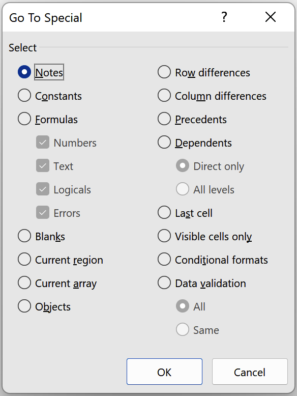
Figure 1-16. The Go To Special dialog box

Formulas, Notes, Conditional Formatting, Constants, and Data Validation

Use these options to find and select cells with the specified contents and attributes.

Select Objects and Selection Pane

These options let you more easily select and manage any objects in your worksheet, such as charts, ink, and shapes.

You can also navigate and select cells using keyboard shortcuts. Here are some of the most useful ones:

Ctrl+Page Up, Ctrl+Page Down

This shortcut navigates to the previous or next worksheet.

Shift+click

This lets you select an adjacent range of cells. Click the first cell, hold down the Shift key, then click the last.

Shift+Arrow keys

This lets you select adjacent rows or columns. Select the first cell, hold down the Shift key, and use the arrow keys to select the adjacent cells.

Ctrl+click or Cmd+click

This lets you select cells that aren’t adjacent. Click the first cell, hold down the Ctrl key if you’re using Excel for Windows or the Cmd key if you’re using Excel for Mac, and then click each cell you want to add to the selection.

Ctrl+A

This selects all the cells in a range, table, PivotTable, or worksheet.

Ctrl+Shift+Arrow keys

This lets you select all the cells in a row or column in a range, table, PivotTable, or worksheet, so Ctrl+Shift+Down, for example, selects the cells in a column.

Discussion

Navigating through spreadsheets and finding cells with specific characteristics can be time-consuming. This recipe helps you work more efficiently using the Find & Select menu options and keyboard shortcuts.

Tip

You can also use hyperlinks to help you navigate to specific locations in your workbook or elsewhere. To insert a link, right-click the cell you want to add it to and choose Link, or select the cell and choose Insert ⇒ Links ⇒ Link.

1.18 Creating a Custom View

Problem

You want to save specific display or print settings—such as hidden rows and columns, filters, or margin widths—so that you can quickly apply them to a worksheet when needed.

Solution

If your workbook doesn’t contain a table, you can save settings in a custom view: a set of settings that applies to a worksheet.

To create a custom view (see Figure 1-17):

1. Go to the worksheet you want to save a custom view for and change the display and print settings you want to save in the Page Layout menu. To open a dialog box showing the complete set of options, click the launcher icon for one of the groups in the ribbon.

2. Choose View ⇒ Workbook Views ⇒ Custom Views to open the Custom Views dialog box.

3. Click Add to open the Add View dialog box, type a name for the custom view, select which options you want to include, and click OK to save the view.

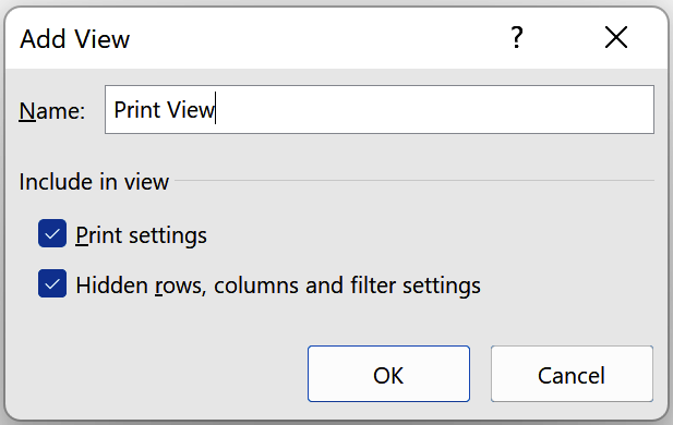
Figure 1-17. The Add View dialog box

To switch to a custom view, go to the worksheet you created the view for, choose View ⇒ Workbook Views ⇒ Custom Views, select the view you wish to display, and click Show.

Warning

Excel disables the Custom Views option if your workbook contains tables, so if you add a table to a workbook containing custom views, you’ll no longer be able to show them.

Discussion

Custom views are a handy way of saving specific display or print settings so you can quickly apply them when needed. You can save views with specific filters, for example, or with settings that you want to apply before printing a worksheet.

1.19 Customizing the Ribbon and Ribbon Tabs

Problem

You want to customize the tabs and commands shown in Excel’s ribbon.

Solution

You can customize Excel’s ribbon using the Customize the Ribbon dialog box. If you’re using Excel for Windows, open the dialog box by choosing File ⇒ Options ⇒ Customize Ribbon or right-clicking the ribbon and selecting Customize the Ribbon. If you’re using Excel for Mac, open it by choosing Excel ⇒ Preferences ⇒ Ribbon & Toolbar.

Generally, you use the Customize the Ribbon dialog box to choose which commands to add to which tabs and which tabs to include. By default, Excel shows you a list of the most popular commands and the ribbon’s main tabs. However, you can change these options to show commands not in the ribbon and all the tabs (see Figure 1-18).

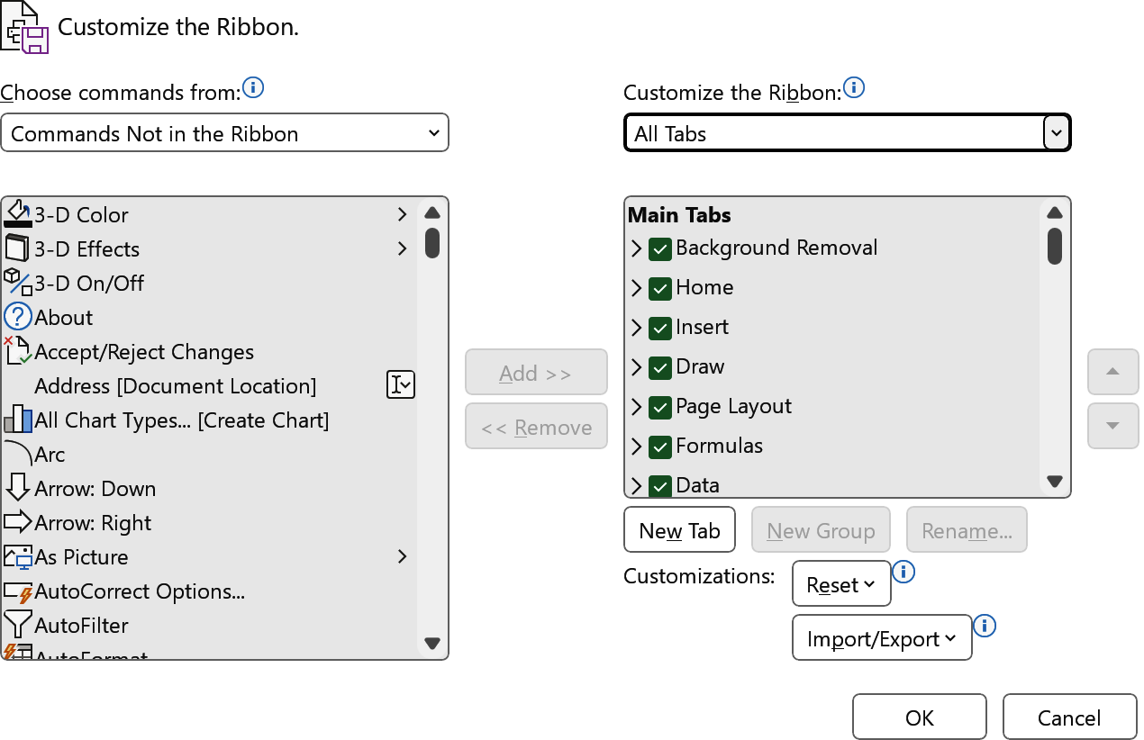
Figure 1-18. The Customize the Ribbon dialog box

Discussion

Customizing Excel’s ribbon is vital when you want to use extra tabs, such as the Developer tab, that aren’t enabled by default. You can also customize the commands shown or reset the ribbon to delete any customizations you no longer need.

Warning

Many recipes in this book refer to ribbon commands and their default tabs, so over-customizing the ribbon may make it harder to follow these recipes.

See Also

You can also add commands to the Quick Access Toolbar; see Recipe 1.20.

1.20 Using the Quick Access Toolbar

Problem

You want to add frequently used commands to an easily accessed toolbar.

Solution

Use the Quick Access Toolbar: a toolbar that gives you quick access to commands.

Depending on your version of Excel, the Quick Access Toolbar appears above the formula bar or in Excel’s title bar. Figure 1-19 shows the Windows version of the toolbar containing AutoSave, Save, Undo, and Redo commands.

Figure 1-19. The Quick Access Toolbar may appear above the formula bar or in the Excel title bar

Tip

The Quick Access Toolbar may not be displayed by default if you’re using Excel for Windows. However, you can show it by right-clicking the ribbon and selecting the Show Quick Access Toolbar.

You can customize the commands shown on the Quick Access Toolbar by clicking the toolbar’s Customize Quick Access Toolbar icon and selecting the commands you want to display in the menu. To see an exhaustive list of commands, select More Commands from the menu, which opens the Customize the Quick Access Toolbar dialog box; this offers the same list of commands as the Customize the Ribbon dialog box (see Recipe 1.19).

If you’re using Excel for Windows, you can also add commands directly from the ribbon by right-clicking the command you want to add and selecting Add to Quick Access Toolbar.

Discussion

The Quick Access Toolbar offers a convenient alternative to Recipe 1.19 since it lets you put all your most commonly used commands in an easily accessible location. You can also use it, for example, to run any macros you’ve created.

1.21 Using the Accessibility Checker

Problem

You have a workbook and want to check for and correct any accessibility issues.

Solution

Excel includes an Accessibility Checker, which you can use to check a workbook for accessibility issues and correct any the tool finds.

To use the Accessibility Checker, choose Review ⇒ Accessibility ⇒ Check Accessibility ⇒ Check Accessibility to open an Accessibility pane. The pane contains a list of inspection results, such as missing object descriptions; click each one to view a list of recommended actions and decide which to apply.

You can also choose Review ⇒ Accessibility ⇒ Check Accessibility ⇒ Options: Accessibility to see Excel’s accessibility options, and Review ⇒ Accessibility ⇒ Check Accessibility ⇒ Accessibility Help to read guidance on making Excel documents more accessible.

Discussion

This recipe introduces you to Excel’s Accessibility Checker, which you can use to check for accessibility issues. It also gives a convenient way of addressing each issue it finds, such as adding alternative text to floating or embedded objects, including charts, shapes, and pictures (see Chapters 12 and 13).

¹ Yes, Word, not Excel.