Designing Autonomous AI

Chapter 1. Sometimes Machines Make Bad Decisions

Why do humans so frequently manage, supervise, step in to assist, or override automated systems? What are the qualities of human decision-making that automated systems cannot replicate? Comparing these strengths and weaknesses helps us design useful AI and avoid thinking that AI is a magical cure-all or complete hype.

I took a trip to Australia and while I was there, a resources company asked for help with their aluminum production process. The company uses an expert system to make automated decisions during the process.

Aluminum is made in large tubs called cells (see Figure 1-1). Aluminum is smelted using a process called electrolysis. In aluminum electrolysis, alumina powder is injected into a cell full of cryolite. Electricity passes through the cryolite, and the resulting reaction produces aluminum. Here’s the problem: it’s almost impossible to tell exactly what’s going on in the cell because the temperature is high enough and the cryolite is corrosive enough to destroy sensors. So experts and automated systems rely on changes in the electrical properties of the cell for feedback. Voltage is how hard the electricity is pushing through the system. Current (measured in amps) is the amount of electricity that flows through the system, and resistance is the amount of opposition the system provides to the flow of electricity.

So standard practice for controlling alumina cells (across the industry, not just at this particular company) is to employ the following two strategies:

• Overfeed the cell (inject more alumina than is likely needed to feed the reaction) until the cell resistance drops. This is a sign that it is time to change strategy.

• Underfeed the cell (inject less alumina than is likely needed to feed the reaction) until the cell resistance rises.

Good aluminum production swings back and forth between these two strategies. The trick is to know when to switch to the opposing strategy. This decision about how to navigate between strategies is nuanced and requires paying attention to how cell resistance changes as well as other variables. This company uses an automated expert system to make this decision for each cell. Expert systems store expert rules (and sometimes equations that describe relationships between variables) to make decisions. I discuss the pros and cons of expert systems in detail in “Expert Systems Recall Stored Expertise”.

In most situations, the expert system makes great decisions about when to transition between strategies, but the boundary between the strategies is fuzzy. In some scenarios, the expert system transitions too early or too late. Both early and late transitions result in effects that degrade aluminum production. When these effects occur, human experts are called in to override the expert system and make the nuanced decisions about when and how to execute the strategies.

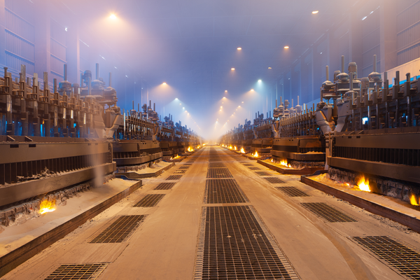
Figure 1-1. Alumina cells for manufacturing aluminum. The example of expert systems in aluminum manufacturing illustrates how automated processes require humans to step in and make decisions when automated systems make bad decisions.

Curiosity Required Ahead

There are a lot of examples in this book! Why are there so many use case examples in this book? Or, put differently, “Why do you keep bringing up so many different engineering processes that I’ve never heard of? It’s a lot to take in!” Here’s my answer: the practice of machine teaching requires curiosity and interest in learning new things above all. I’ve been asked to formulate autonomous AI designs for all kinds of machines, systems, and processes, most of which I had never heard of in my life (including aluminum smelting). Sometimes, I was asked to come up with these designs very quickly, in hours, or even minutes. This was made possible by my intense curiosity about engineering processes and by the framework that I teach in this book. As you read through the examples in this book, hopefully you will appreciate that in order to design effective autonomous AI, you need to have an appetite for learning.

Math, Menus, and Manuals: How Machines Make Automated Decisions

If you want to design brains well, you first need to understand how automated systems make decisions. You will use this knowledge to compare techniques and decide when autonomous AI will outperform existing methods. You will also combine automated decision-making with AI to design more explainable, reliable, deployable brains. Though there are many subcategories and nuances, automated systems rely on three primary methods to make decisions: math, menus, and manuals.

Control Theory Uses Math to Calculate Decisions

Control theory uses mathematical equations to calculate the next control action, usually based on feedback, using well-understood mathematical relationships. When you do this, you must trust that the math describes the system dynamics well enough to use it to calculate what to do next. Let me give you an example. There’s an equation that describes how much space a gas will take up based on its temperature and pressure. It’s called the ideal gas law. So if we wanted to design a brain that controls a valve that inflates party balloons, we could use this equation to calculate how much to adjust the valve open and closed to inflate balloons to a particular size.

In the example above, we rely on math to describe what will happen so completely and accurately that we don’t even need feedback. Controlling based on equations like this is called open loop control because there is no closed feedback loop telling us whether our actions achieved the desired results. We trust the equation so much that we don’t even need feedback. But what if the equation doesn’t completely describe all of the factors that affect whether we succeed or not? For example, the ideal gas law doesn’t model high-pressure, low-temperature gases, dense gases, or heavy gases well. Even when we control responding to feedback, limitations of the mathematical model might lead to bad decisions.

I see the history of control theory as an evolution of capability where each control technology can do things that previous control technologies could not. The U.S. Navy invented the Proportional Integral Derivative (PID) controller to automatically steer ship rudders and control ship headings (the direction the ship is pointing). Imagine that a ship is pointing in one direction and the captain wants to change headings to point the ship in a different direction, as shown in Figure 1-2.

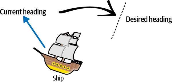
Figure 1-2. Ship changing heading.

The controller uses math to calculate how much to move the rudder based on feedback it gets from its last action. There are three numbers that determine how the controller will behave: the P, the I, and the D constant. The P constant moves you toward the target, so for the ship, the P constant makes sure that the rudder action causes the ship to move towards its new heading. But what if the controller keeps turning the rudder and the ship sweeps right past the target heading? This is what the I constant is for. The I constant tracks how much total error you have in the system and keeps you from overshooting or undershooting the target. The D constant ensures that you arrive at the target destination smoothly instead of abruptly. So a D in the ship controller would make it more likely that the ship will decelerate and arrive more precisely to its destination heading.

A ship with a P controller (no I and no D) might overshoot the target, sweeping the boat past the new heading. After the ship sweeps past the target, you’ll need to turn it back. The leftmost diagram in Figure 1-3 shows what this might look like. The horizontal line represents the destination heading. A PI controller will more quickly converge on the target because the I term makes sure that you overshoot the target as little as possible. The PD controller approaches the target more smoothly, but takes longer to reach it.

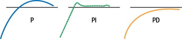
Figure 1-3. Example behaviors of various controllers.

The PID controller can be very effective and you can find it in almost every modern factory and machine, but it can confuse disturbances and noise for events that it needs to respond to. For example, if a PID controller controlled the gas pedal on your car, it might confuse a speed bump (which is a minor and temporary disturbance) for a hill which requires significant acceleration. In this case, the controller might overaccelerate and exceed the commanded speed, then need to slow down.

The feedforward controller separately measures and responds to disturbances, not just the variable you are controlling. In contrast to PID feedback control, Jacques Smuts writes:

feedforward control acts the moment a disturbance occurs, without having to wait for a deviation in process variable. This enables a feedforward controller to quickly and directly cancel out the effect of a disturbance. To do this, a feedforward controller produces its control action based on a measurement of the disturbance.

When used, feedforward control is almost always implemented as an add-on to feedback control. The feedforward controller takes care of the major disturbance, and the feedback controller takes care of everything else that might cause the process variable to deviate from its set point.¹

In our cruise control example, this means that the controller can better tell the difference between a speed bump and a hill by measuring and responding to the disturbance (the change in road elevation) instead of measuring and responding only to the change in the vehicle’s speed. See Figure 1-4 for an example showing how much better feedback with feedforward control responds to a disturbance than feedback control alone.

The more sophisticated feedforward controller has limitations too. Both PID and feedforward controllers can only control for one variable at a time for one goal per feedback loop. So you’d need two feedback/feedforward loops, for example, if you needed to control both the gas pedal and the steering wheel of the car. And neither of those loops can both maximize gas mileage and maintain constant speed at the same time.

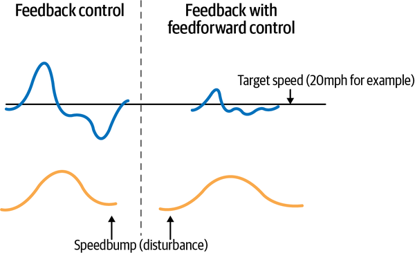
Figure 1-4. Comparing how a car controlled by PID feedback control responds to a speed bump versus one controlled by feedforward; the fluctuation in speed is much smaller with feedforward control.

So what happens if you need to control for more than one variable or pursue more than one goal? There are ways to solve this, but in real life we often see people create separate feedback loops that can’t talk to each other or coordinate actions. So in the same way that humans duplicate work and miscalculate what to do when we don’t coordinate with each other, separate control loops don’t manage multiple goals well and often waste energy.

Enter the latest in the evolution of widely adopted control systems: model predictive control (MPC). MPC extends the capability of PID and feedforward to control for multiple inputs and outputs. Now, the same controller can be used to control multiple variables and pursue multiple goals. The MPC controller uses a highly accurate system model to try various control actions in advance and then choose the best action. This control technique actually borrows from the second type of automated decision-making (menus). It has many attractive characteristics, but lives or dies by the accuracy of the system model, or the equations that predict how the system will respond to your actions. But real systems change: machines wear, or equipment is replaced, the climate changes, and this can make the system model inaccurate over time. Many of us have experienced this in our vehicles. As the brakes wear, we need to apply the brakes earlier to stop. As the tires wear, we can’t drive as fast or turn as sharply without losing control. Since the MPC uses the system model to look ahead and try potential actions, an inaccurate model will mislead it to decide on actions that won’t work well on the real system. Because of this, many MPC systems that were installed, particularly in chemical plants in the 1990s, were later decommissioned when the plants drifted from the system models. The MPC controllers that relied heavily on these system models in order to be accurate no longer controlled well.

In 2020, McKinsey QuantumBlack built an autonomous AI to help steer the Emirates Team New Zealand sailing team to victory by controlling the rudder of their boat. This AI brain can input many, many variables including ones that math-based controllers can’t, like video feeds from cameras and categories (like forward, backward, left, right). It learns by practicing in simulation and acquires creative strategies to pursue multiple goals simultaneously. For example, in its experimentation and self-discovery, it tried to sail the boat upside down because for a while, during practice in simulation, it seemed like a promising approach to accomplish sailing goals.

Control theory uses math to calculate what to do next, the techniques to do this continuously evolve, and autonomous AI is simply an extension of these techniques that offers some really attractive control characteristics such as the ability to control for multiple variables and track toward multiple goals.

When Should You Use Control Theory to Make Decisions?

• Use control theory when you need reliable, predictable control of processes that you can measure well.

• Use control theory when you understand the system dynamics well and can express them in mathematical terms.

Limitations of Control Theory

• Controllers that use math to make decisions rely heavily on the mathematical model. If you can’t model the system well with math, you can’t control it well with control theory.

• The settings on controllers make them work well for linear systems, but not as well when there are nonlinear relationships between the variables.

• The controller will not change its behavior unless human experts retune the constants.

Optimization Algorithms Use Menus of Options to Evaluate Decisions

Optimization algorithms search a list of options and select a control action using objective criteria. Think about the way optimization works, like selecting options from a menu. For example, an optimization system might list all possible routes to deliver a package from manufacturing point A to delivery point B, then select sequential routing decisions by sorting the shortest route to the top of the list of options. You might come up with different control actions if you sort for the shortest trip duration. In this example, the route distance and the trip durations are the objective criteria (the goals of the optimization). Imagine playing tic-tac-toe this way. Tic-tac-toe is a simple two player game played on a grid where you place your symbol, an X or an O, in squares on the grid and you win when you are the first player to occupy three squares in a row with your symbol. If you want to play the game like an optimization algorithm, you could use the following procedure:

1. Make a list of all squares (there are 9, see Figure 1-5 for an example).

2. Cross out (from the list) the squares that already have an X or an O in them.

3. Choose an objective to optimize for. For example, you might decide to make moves based on how many blank squares there are adjacent to each square. This objective gives you the most flexibility for future moves. This is why many players choose the center square for their first move (there are 8 squares adjacent to the middle square).

4. Sort your options based on the objective criteria.

5. The top option is your next move. If there are multiple moves with the exact same objective criteria score, choose one randomly.

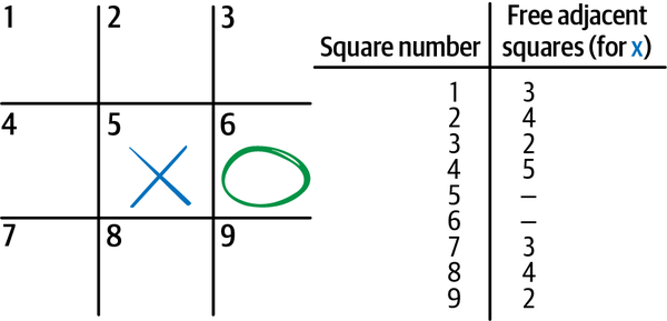
Figure 1-5. Diagram of tic-tac-toe board showing X making the first move, O making the second move, the number of adjacent squares that are open or under X’s control for each option available for X’s next move, and a list that tracks the attributes of each square.

This exercise shows the first limitation of optimization algorithms. They don’t know anything about the task. This is why you need to choose a square randomly if there are multiple squares with the same objective score at the top of your search. Claude Shannon, one of the early pioneers of AI, talked about this in his famous 1950 paper about chess-playing AI.² He observed that there were two ways to program a chess AI. He labeled them System A and System B. System A, which is actually the third method of automated decision-making (manuals), programs chess strategies. These rules and exceptions are difficult to manage and update, but they express understanding of the game. System B, which is optimization, searches possible legal chess moves with a single easy-to-maintain algorithm, but has no actual understanding of the concepts or strategies of chess.

Strategy Versus Search

I believe that strategy is one of the missing key ingredients of AI research. I think that Claude Shannon (an early pioneer of AI) would agree with me. Strategy is a key way that we make sense of the world, and Shannon predicted a long time ago that there would be friction about whether to use strategy or search options, as shown in Figure 1-6.

Figure 1-6. Two approaches for making complex sequential decisions.

Solutions Are like Points on a Map

Optimization algorithms are like explorers searching the surface of the earth for the highest mountain or the lowest point. The solutions to problems are points on the map where, if you arrive, you achieve some good outcome. If your goal is altitude, you are looking for the peak of Mt. Everest, at 8,848 meters above sea level (see Figure 1-7 for a map of Earth relief by altitude in relation to sea level). If your goal is finding the location that is most packed with people (population density), you are looking for the Chinese island of Macau, which has a population density of 21,081 people/km² (see Figure 1-8 for a map of Earth relief by population density). If you’re looking for the coldest place on earth on average, then you’re looking for Vostok Station, Antarctica.

Now, imagine that you are an optimization algorithm searching the earth for the highest peak. One way to ensure that you find the highest peak is to set foot on every square meter of earth, take measurements at each point and then, when you are done, sort your measurements by altitude. The highest point on earth will now be at the top of your list.

Since there are 510 million square kilometers of land mass on earth, it would take many, many lifetimes to get your answer.³ This method is called brute force search and is only feasible when the geographical search area of possible decisions is very small (like in the game tic-tac-toe). For more complex problem geographies, we need another method.

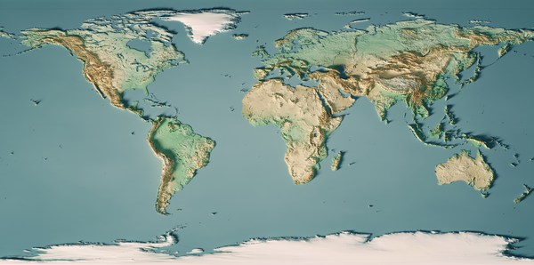
Figure 1-7. World map relief by altitude.

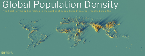
Figure 1-8. World map relief by population density.

A more efficient way to search the earth for the highest peak is to walk the earth and only take steps in the direction that slopes upward the most. Using this method, you can avoid exploring much of the geography by only traveling uphill. In optimization, this class of methods is called gradient-based methods because the slope of a hill is called a grade or a gradient. There are two challenges with this method. The first is that, depending on where you start your search exploration, you could end up on a tall mountain that is not the highest point on earth. If you start your search in Africa, you could end up on Mt. Kilimanjaro (not the world’s tallest peak). If you start in North America, you could end up on top of one of the mountains in the Rocky Mountain range. You could even end up on a much lesser peak because once you ascend any peak using this search method, you cannot descend back down any hill. Figure 1-9 demonstrates how this works.

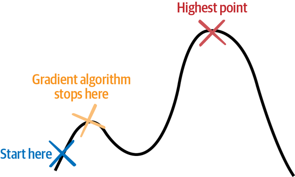
Figure 1-9. A gradient-based algorithm will stop searching in relation to the highest point on a curve.

The second limitation of this method is that it can only be used in situations where you can calculate the slope of the ground where you walk. If there are gaps in the terrain (think vertical drops or bottomless pits), it is not possible to calculate the slope (technically it’s infinite) at the vertical drops, so you can’t use gradient-based optimization methods to search for solutions in that space. See Figure 1-10 for examples of solution terrain that gradient algorithms cannot search.

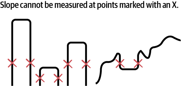
Figure 1-10. These examples of function curves cannot be searched using gradient-based methods.

Now, imagine if you employed multiple explorers to start at different places in the landscape and search for the highest point. After each step, the explorers compare notes on their current altitude and elevation and use their combined knowledge to better map the earth. That might lead to a quicker search and avoid all explorers getting stuck in a high spot that is not the peak of Mt. Everest. These and other innovations allow optimization algorithms to more efficiently and effectively explore more kinds of landscapes, even the ones shown in Figure 1-10. Many of these algorithms are inspired by processes in nature. Nature has many effective ways of exploring thoroughly, much like water flowing over a patch of land. Here are a few examples:

Evolutionary algorithms

Inspired by Darwin’s theory of natural selection, evolutionary algorithms spawn a population of potential solutions decisions, test how well each of the solutions in the population achieve the process goals, kill off the ineffective solutions, then mutate the population to continue exploring.

Swarm methods

Inspired by how ants, bees, and particles swarm, move, and interact, these optimization methods explore the solution space with many explorers that move along the landscape and communicate with each other about what they find. Figure 1-11 illustrates how these explorers work.

Tree methods

These methods treat potential solutions as branches on trees. Imagine a choose-your-own-adventure novel (and other interactive fiction) that asks you to decide which direction to take at a certain point in the story. The decisions proliferate with the number of options at each decision point. Tree-based methods use various techniques to search the tree efficiently (not having to visit each branch) for solutions. Some of the more well known tree methods are branch and bound and Monte Carlo tree search (MCTS).

Simulated annealing

Inspired by the way that metal cools, simulated annealing searches the space using different search behavior over time. All metals have a crystalline structure that cools in a common way. That structure changes more when the metal is hotter and less when cooler. Annealing is a process by which a material like metal is heated above its recrystalization temperature and then slowly cooled in order to render it more malleable for the next steps in various industrial processes. This algorithm imitates that process. Simulated annealing casts a wide search net at first (exploring more), then becomes more sure that it’s zeroing in on the right area (exploring less) over time.

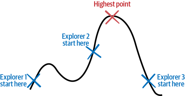
Figure 1-11. Some optimization algorithms use multiple coordinated explorers.

Solving the Game of Checkers

There is a scene in the movie The Matrix where the main character Neo finds a child, dressed as a Shaolin monk, bending a spoon with his mind. Seeing that Neo is perplexed, the child explains that there is no spoon. Neo and the child are in a manipulative virtual digital world that a rogue machine AI conjured to entrap humans in their minds. The child is manipulating the imaginary code-based world that their human minds occupy.

I feel similarly about making the perfect sequential decision while performing a complex task. Optimization experts call these “best possible decisions” (like Mt. Everest or the highest topography points in Figures 1-9 and 1-11) global optima. Optimization algorithms promise the possibility of reaching global optima for every decision, but this is not how it works in real, complex systems. For example, there is no “perfect move” during a chess match. There are strong moves, creative moves, weak moves, surprising moves, but no perfect moves for winning a particular game. That is, unless you’re playing checkers.

In 2007, after almost 20 years of continuously searching the space with optimization algorithms on powerful computers, researchers declared checkers solved. Checkers is roughly 1 million times more complex than Connect Four, with 500 billion billion possible positions (5 × 10²⁰). I spoke with Dr. Jonathan Schaeffer, one of the lead researchers on the project, and this is what he told me:

We proved that perfect play leads to a draw. That is not the same as knowing the value of every position. The proof eliminates vast portions of the search. For example, if we find a win, the program does not bother looking at the inferior moves that yield a draw or a loss. Thus, if you set up a position that occurs in one of those drawing/losing lines, the program might not know its solved value.

So why don’t we just solve our industrial problems like checkers? Besides the fact that it took optimization algorithms 20 years to solve checkers, most real problems are more complex than that, and the checkers space is not completely explored, even after all that computation. Remember the tree based optimization methods above? Well, one way that computer scientists devised to measure the complexity of tasks is to count the number of possible options at the average branch of the tree. This is called the branching factor. The branching factor for checkers is 2.8, which means on average there are about 3 possible moves for any turn during a checkers game. This is mostly due to the forced capture rule in checkers. In a capture position, the branching factor is slightly larger than 1. In a noncapture position, the branching factor is approximately 8. Branching factors for some of the most popular board games are summarized in Table 1-1.

Table 1-1. Branching factors for common games

Game	Branching factor
Checkers	2.8
Tic-tac-toe	4
Connect Four	4
Chess	35
Go	250

Then there’s uncertainty. One very convenient aspect of games like checkers and chess is that things always happen exactly the way you want them to. For example, if I want to move my bishop all the way across the board (the chess term for putting the bishop on this cross-board highway of the longest diagonal, as illustrated in Figure 1-12, is fiancetto), I can be certain that the bishop will make it all the way to G7 as I intended. But in the real life war campaigns that chess was modeled after, an offensive to take a certain hill is not guaranteed to succeed, so our bishop might actually land at F6 or E5 instead of our intended G7. This kind of uncertainty about the success of each move will likely change our strategy. I’ll talk more about uncertainty in a minute.

So for real problems (such as bending spoons in the Matrix), when it comes to finding optimal solutions for each move you need to make, there is indeed no spoon.

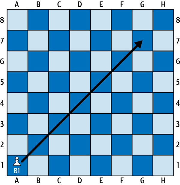
Figure 1-12. Bishop moving from A1 to G7 on a chess board.

Reconnaissance

Reconnaissance just means scouting ahead. You can’t explore the entire space ahead of time, but in some situations you can scout out local surrounding areas a few moves in advance. For example, model predictive control (MPC) looks at least one move in advance when making decisions. To do this, you need a model that will accurately predict what will happen after you make a decision.

Most of the AI that performs this kind of reconnaissance uses it in situations with discrete outcomes at each step. This is true for games like chess and Go, but it’s also true for decisions in manufacturing planning and logistics. Imagine determining which machines to make products on or which shipment carrier to use for a delivery.

Autonomous AI like AlphaChess, AlphaGo, and AlphaZero can’t make good decisions without scouting many moves ahead. These AI use Monte Carlo tree search (MCTS) to navigate large spaces like chess, shogi, and Go, as shown in Figure 1-13.

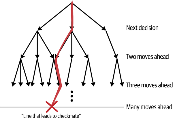
Figure 1-13. A line of moves leading to a winning outcome expressed on a tree of lookahead options.

You can use trees to search many moves ahead. The first set of branches on the tree represent options for your next move and each further branch on the tree represents further future moves. The idea is to keep looking at more future moves until you reach the end of the game. When you do, there will be paths through the branches (called lines in chess) that lead to winning outcomes and others that lead to losing outcomes. If you can make it that far through the search, you’ll have lots of winning lines that you can pursue. The average chess game lasts 20 to 40 moves and the tree representing any one of those games has more branches than the number of atoms in the universe. That doesn’t mean that you shouldn’t use look ahead moves though. There are many ways to pare down the number of branches that you need to examine to get to winning outcomes.

MCTS randomly searches branches on the tree for as long as you have time and compute power to spare. The World Chess Federation (commonly referred to by its French name, Fédération Internationale des Échecs [FIDE]) mandates 90 minutes for each player’s first 40 moves, then 30 minutes total for both players to finish the game. AlphaZero uses 44 CPU computer cores to randomly search about 72,000 tree branches for each move. Depending on chance, the algorithm might or might not find a winning line during the search between each of its moves.

Both professional chess and Go players say that the AI has an “alien playing style” and I say that is because of the randomness of MCTS. You see, when the search algorithm finds a line, it chases it and will do absolutely anything (no matter how unorthodox or sacrificial) to follow it. Then, depending on the opponent’s play, the algorithm may pick up a new line with seemingly disjointed unorthodox moves and sacrifices. Some of these lines are brilliant, creative, and thrilling to watch but are also at times erratic. Before we move on, let’s give credit where it’s due: AlphaZero beat the de facto standard AI in machine chess (Stockfish) 1,000 games to zero in 2019.

Humans look ahead, but not in this way. Psychologists’ research on chess players shows that expert chess players focus on only a small subset of total pieces and review an even smaller subset of tree branches when scouting ahead for options.⁴ How are they able to look many moves ahead without randomly exploring so many options? They’re biased. Many options don’t make sense as strong chess moves, others don’t make sense based on the strategy that the player is using, others still don’t make sense based on the strategy that the opponent is using. I suggest that a promising area of research is using human expertise and strategy to bias the tree search (only explore options that match the current strategy).

What About Uncertainty?

Using optimization algorithms to look ahead depends upon discrete actions and certainty about what will happen when you take an action. Many problems that you work on will have to deal with uncertainty and continuous actions. Almost every logistics and manufacturing problem that I’ve designed a brain for displays seasonality. Much the same way that tides ebb and flow and the moon waxes and wanes in the sky, seasonal variations follow a periodic pattern. Here’s some examples of seasonal patterns of uncertainty:

• Traffic

• Seasonal demand

• Weather patterns

• Wear and replacement cycle for parts

The good news is that this uncertainty is not random. Uncertainty blurs scenarios according to predefined patterns, much the same way that fuzzy boundaries blur the edges of the shapes in Figure 1-14.

Figure 1-14. Blurry circles.

Each of the shapes is like a scenario for one of the problems you solve. For traffic, there are heavy traffic scenarios (like during commute hours and after an accident) and there are scenarios with lighter traffic. But the boundaries for these scenarios are blurry. Sometimes morning commute traffic starts earlier, sometimes later. But these scenarios and the uncertainty that blurs them do obey patterns. We will need more than optimization algorithms to recognize and respond to these patterns and make decisions through the uncertainty that sits on top of these patterns.

You can spend an entire professional or academic career learning about optimization methods, but this overview should provide the context you need to design brains that incorporate optimization methods and outperform optimization methods for decision-making about specific tasks and processes. If you’d like to learn more about optimization methods, I recommend Numerical Optimization by Nocedal and Wright (Springer).

When Should You Use Optimization Algorithms to Make Decisions?

• When you don’t have experience or mathematical formulas to tell you what to do

• When the search landscape is very large or where part of the search space is unexplored

• When there are many rules for decision-making (constraints) that need to be followed

• When the value to you of having a better answer (however slight) is significant

Limitations of Optimization

• Optimization algorithms encapsulate no understanding of the system or the skills and strategies required to optimize the system.

• Optimization algorithms require significant time and computational resources to search through options for the decisions they choose.

Expert Systems Recall Stored Expertise

Expert systems look up control actions from a database of expert rules—essentially, a complex manual. This provides compute-efficient access to effective control actions, but creating that database requires existing human expertise—after all, you have to know how to bake a cake in order to write the recipe. Expert systems leverage understanding of the system dynamics and effective strategies to control the system, but they require so many rules to capture all the nuanced exceptions that they can be cumbersome to program and manage.

Let’s use an example from an HVAC system like the one that might control the temperature in an office building. The system uses a damper valve that can be opened to let in fresh air or closed to recycle air. The system can save energy by recycling air at times of day when the price of energy is high or when the air is very cold and needs to be heated up. However, recycling too much air, especially when there are many people in the building, decreases air quality as carbon dioxide builds up.

Let’s say we implement an expert system with two simple rules that set the basic structure:

• Close the damper to recycle air when energy is expensive or when air is very cold (or very hot).

• Open the damper to let in fresh air when the air quality is approaching legal limits.

These rules represent the two fundamental strategies for controlling the system. See Figure 1-15 for a diagram of how the damper works.

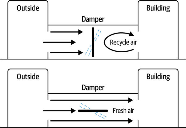
Figure 1-15. How a damper valve in a commercial HVAC system recycles and freshens air.

The first control strategy is perfect for saving money when energy is expensive and when temperatures are extreme. It works best when building occupancy is lower. The second strategy works well when energy is less expensive and building occupancy is high.

But we’re not done yet. Even though the first two rules in our expert system are simple to understand and manage, we need to add many more rules to execute these strategies under all possible conditions. The real world is fuzzy, and every rule has hundreds of exceptions that would need to be codified into an expert system. For example, the first rule tells us that we should recycle air when the energy is expensive and when the air temperature is extreme (really hot or cold). How expensive should the energy be in order to justify recycling air? And how much should you close the damper valve to recycle air? Well, that depends on the carbon dioxide levels in the rooms and on the outdoor temperature. It’s nuanced—and the right answer depends on the surface of the landscape defined by the relationships between energy prices, outdoor air temperatures, and number of people in the building.

if (temp > 90 or temp < 20) and price > 0.15: # Recycle Air
	if temp < 00 and price > 0.17:
		valve = 0.1
	elif temp < 10 and price > 0.17:
		valve = 0.2
	elif temp < 20 and price > 0.17:
		valve = 0.3

The code above shows some of the additional rules required to effectively implement two HVAC control strategies under many different conditions.

Expert systems are like maps of the geographic terrain: recorded exploration drawn based on previous expeditions. They hold a special place in the history of AI: in fact, they comprised most of its second wave. The term artificial intelligence was coined in 1956 at a conference of computer scientists at Dartmouth College. The first wave of AI used symbolic (human-readable) representations of problems, logic, and search to reason and make decisions. This approach is often called symbolic AI.

The second wave of AI primarily comprised expert systems. For some time, the hope was that the expert system would serve as the entire intelligent system even to the point of intelligence comparable to the human mind. Folks as famous as Marvin Minsky, regarded as the “Godfather of AI,” claimed this. From a research perspective, much of the exploration of what an expert system was and could be was considered complete. Even, so widespread disappointment in the capability of these systems was recorded.

A big reason why expert systems died is the knowledge acquisition bottleneck. This is another insight from my interview with Jonathan Schaeffer. Expert systems use knowledge gleaned from humans, but how do you get the knowledge from the humans in terms that can be easily mapped to code? Not so easy, in general! This is why early expert systems died. They were too brittle. Getting the knowledge was hard. Identifying and handling all the exceptions is harder. Chess grandmaster Kevin Spraggett says it well: “I spent the first half of my career learning the principles for playing strong chess and the second half learning when to violate them.”

A long AI “winter” descended amid disappointment that the expert system was not sufficient to replicate the intelligence of the human mind (the field of AI research calls the hypothetical ability of an AI to understand and learn intellectually, as a human could, artificial general intelligence, or AGI). Perception was missing, for example. Expert systems can’t perceive complex relationships and patterns in the world the way we see (identify objects based on patterns of shapes and colors), hear (detect and communicate based on patterns of sounds), and predict (forecast outcomes and probabilities based on correlations between variables). We also need a mechanism to handle the fuzzy exceptions that trip up expert systems. So expert systems silently descended underground to be used in finance and engineering, where they shine at making high-value decisions to this day.

The current “summer” of AI swung the pendulum all the way in the opposite direction, as illustrated in Figure 1-16. The expert system was shunned in favor of perception, then in favor of learning algorithms that make sequential decisions.

Note

We now have an opportunity to combine the best of expert systems with perception and learning agents in next-generation autonomous AI! Expert systems can codify the principles that Spraggett was talking about and the learning parts of autonomous AI can identify the exceptions by trial and error.

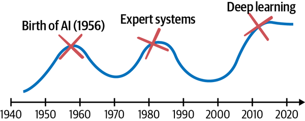
Figure 1-16. Timeline of the history of AI.

If you would like to learn more about how expert systems fit into the history of AI, I highly recommend Luke Dormehl’s Thinking Machines: The Quest for Artificial Intelligence and Where It’s Taking Us Next (TarcherPerigee), an accessible and relevant survey of the history of AI. If you would like to read details about a real expert system, I recommend this paper on DENDRAL, widely recognized as the first “real” expert system.

Fast forward to today and we find expert systems embedded in even the most advanced autonomous AI. An expert once described to me an autonomous AI that was built to control self-driving cars. Deep in the logic that orchestrates learning AI to perceive and act while driving are expert rules that take over during safety-critical situations. The learning AI perceives and makes fuzzy, nuanced decisions, but the expert system components do what they are really good at, too: taking predictable action to keep the vehicle (and people) safe. This is exactly how we will use math, menus, and manuals when we design brains. We will assign decision-making technology to best execute each decision-making skill.

When Should You Use Expert Systems to Make Decisions?

• When you have a lot of experience exploring the space, know what to do for many different scenarios, and can express desired actions and in terms of rules and/or strategies

• When you have many constraints that must be obeyed (as with optimization algorithms)

• When you need to explain your decisions but you don’t have a mathematical model that you trust enough to use its calculations to determine actions

Limitations of Expert Systems

• Expert systems are limited by knowledge from previous exploration.

• Maintaining the rules—and all the exceptions—in the knowledge base is tedious and error-prone.

Now that I’ve discussed each method that machines use to make automated decisions, you can see that each method has strengths and weaknesses. In some situations, one method might be a clear and obvious choice for automated decisions. In other applications, another method might perform much better. Now, we can even consider mixing methods to achieve better results, the way that MPC does. It makes better control decisions by mixing math with manuals in the form of a constraint optimization algorithm. But first, let’s take a look at the capabilities of autonomous AI.

¹ Jacques Smuts, “A Tutorial on Feedback Control,” Control Notes: Reflections of a Process Control Practitioner, January 17, 2011, https://blog.opticontrols.com/archives/297.

² Claude E. Shannon, “Programming a computer for playing chess,” Philosophical Magazine, 7th series, 41, no. 314 (March 1950): 256-75.

³ George Heineman’s Learning Algorithms (O’Reilly) provides details on how to benchmark these algorithms.

⁴ W. G. Chase and H. A. Simon, “Perception in Chess,” Cognitive Psychology 4, no. 1 (1973): 55-81. https://dx.doi.org/10.1016/0010-0285(73)90004-2