Deep Learning for Finance

Chapter 4. Linear Algebra and Calculus for Deep Learning

Algebra and calculus are integral parts of data science. Machine learning and deep learning algorithms are mostly based on algebra and calculus techniques. This chapter introduces some key topics in a way that everyone can understand.

Algebra is the study of operations and relational rules, as well as the constructions and ideas that result from them. Algebra covers topics such as linear equations and matrices. You can consider algebra as the first step toward calculus.

Calculus is the study of curve slopes and rates of change. Calculus covers topics such as derivatives and integrals. It is heavily used in many fields such as economics and engineering. Many learning algorithms rely on the concepts of calculus to perform their complex operations.

The distinction between the two is that while calculus works with ideas of change, motion, and accumulation, algebra deals with mathematical symbols and the rules for manipulating those symbols. Calculus focuses on the characteristics and behavior of changing functions, while algebra offers the foundation for solving equations and comprehending functions.

Linear Algebra

Algebra encompasses various mathematical structures, including numbers, variables, and operations like addition, subtraction, multiplication, and division. Linear algebra is a fundamental branch of algebra that deals with vector spaces and linear transformations. It is heavily used in machine learning and deep learning for tasks such as data preprocessing, dimensionality reduction, and solving systems of linear equations. Matrices and vectors are central data structures in linear algebra, and operations like matrix multiplication are common in various algorithms.

Vectors and Matrices

A vector is an object that has a magnitude (length) and a direction (arrowhead). The basic representation of a vector is an arrow with coordinates on the axis. But first, let’s see what an axis is.

The x-axis and y-axis are perpendicular lines that specify a plane’s boundaries and the locations of different points within them in a two-dimensional Cartesian coordinate system. The x-axis is horizontal and the y-axis is vertical.

These axes may represent vectors, with the x-axis representing the vector’s horizontal component and the y-axis representing its vertical component.

Note

In time series analysis, the x-axis is typically the time step (hours, days, etc.), and the y-axis is the value at the respective time step (price, return, etc.).

Figure 4-1 shows a simple two-dimensional Cartesian coordinate system with both axes.

The two-dimensional Cartesian coordinate system uses simple parentheses to show the location of different points following this order:

• Point coordinates = (x, y)

• The variable x represents the horizontal location

• The variable y represents the horizontal location

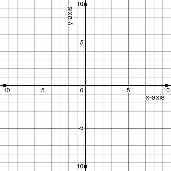
Figure 4-1. A two-dimensional Cartesian coordinate system

Therefore, if you want to draw point A, which has (2, 3) as coordinates, you are likely to look at a graph from point zero, move two points to the right, and from there, move three points upward. The result of the point should look like Figure 4-2.

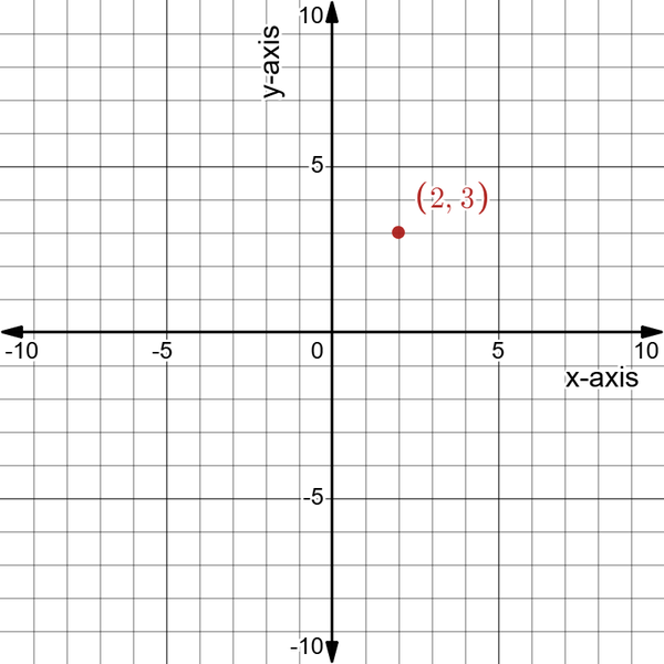
Figure 4-2. The location of A on the coordinate system

Let’s now add another point and draw a vector between them. Suppose you have point B with (4, 5) as coordinates. Naturally, as the coordinates of B are higher than the coordinates of A, you would expect vector AB to be upward sloping. Figure 4-3 shows the new point B and vector AB.

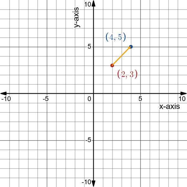
Figure 4-3. Vector AB joining points A and B together in magnitude and direction

However, having drawn the vector using the coordinates of both points, how would you refer to the vector? Simply put, vector AB has its own coordinates that represent it. Remember that the vector is a representation of the movement from point A to point B. This means the two-point movement along the x-axis and the y-axis is the vector. Mathematically, to find the vector, you should subtract the two coordinate points from each other while respecting the direction. Here’s how to do that:

• Vector AB means that you are going from A to B; therefore, you need to subtract the coordinates of point B from the coordinates of point A:

  $\begin{array}{c}\overrightarrow{AB}=\langle 4-2,5-3\rangle \hfill \\ \overrightarrow{AB}=\langle 2,2\rangle \hfill \end{array}$

• Vector BA means that you are going from B to A; therefore, you need to subtract the coordinates of point A from the coordinates of point B:

  $\begin{array}{c}\overrightarrow{BA}=\langle 2-4,3-5\rangle \hfill \\ \overrightarrow{BA}=\langle -2,-2\rangle \hfill \end{array}$

To interpret the AB and BA vectors, you need to think in terms of movement. Vector AB represents going from point A to point B, two positive points horizontally and vertically (to the right and upward, respectively). Vector BA represents going from point B to point A, two negative points horizontally and vertically (to the left and downward, respectively).

Note

Vectors AB and BA are not the same thing even though they share the same slope. But what is a slope anyway?

The slope is the ratio of the vertical change between two points on the line to the horizontal change between the same two points. You calculate the slope using this mathematical formula:

$\begin{array}{c}Slope=\frac{\left(\Delta Y\right)}{\left(\Delta X\right)}\hfill \\ Slopeof\overrightarrow{AB}=\frac{2}{2}=1\hfill \\ Slopeof\overrightarrow{BA}=\frac{-2}{-2}=1\hfill \end{array}$

If the two vectors were simply lines (with no direction), then they would be the same object. However, adding the directional component makes them two distinguishable mathematical objects.

Figure 4-4 sheds more light on the concept of the slope, as x has shifted two points to the right and y has shifted two points to the left.

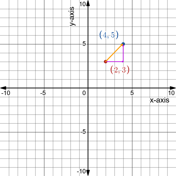
Figure 4-4. The change in x and the change in y for vector AB

Note

A vector that has a magnitude of 1 is referred to as a unit vector.

Figure 4-5 shows the change in x and the change in y in the case of vector BA.

Figure 4-5. The change in x and the change in y for vector BA

Researchers typically use vectors as representations of speed, especially in engineering. Navigation is one field that heavily relies on vectors. It allows navigators to determine their positions and plan their destinations. Naturally, magnitude represents speed and the direction represents the destination.

You can add and subtract vectors from each other and from scalars. This allows for a shift in direction and magnitude. What you should retain from the previous discussion is that vectors indicate directions between different points on the axis.

Note

A scalar is a value with magnitude but no direction. Scalars, as opposed to vectors, are used to represent elements, like temperature and prices. Basically, scalars are numbers.

A matrix is a rectangular array containing numbers and organized in rows and columns.¹ Matrices are useful in computer graphics and other domains as well as to define and manipulate linear systems of equations. What differentiates a matrix from a vector? The simplest answer is that a vector is a matrix with a single column or a single row. Here’s a basic example of a 3 × 3 matrix:

$\left[\begin{array}{ccc}5& 2& 9\\ -8& 10& 13\\ 1& 5& 12\end{array}\right]$

The size of a matrix is the number of rows and columns it contains. A row is a horizontal line, and a column is a vertical line. The following representation is a 2 × 4 matrix (i.e., two rows by four columns):

$\left[\begin{array}{cccc}5& 2& 1& 3\\ -8& 10& 9& 4\end{array}\right]$

The following representation is a 4 × 2 matrix (i.e., four rows by two columns):

$\left[\begin{array}{cc}5& 2\\ -8& 10\\ 8& 22\\ 7& 3\end{array}\right]$

Note

Matrices are heavily used in machine learning. Rows generally represent time and columns represent features.

The summation of different matrices is straightforward but must be used only when the matrices match in size (which means they have the same number of columns and rows). For instance, let’s add the following two matrices:

$\left[\begin{array}{cc}1& 2\\ 5& 8\end{array}\right]+\left[\begin{array}{cc}3& 9\\ 1& 5\end{array}\right]=\left[\begin{array}{cc}4& 11\\ 6& 13\end{array}\right]$

You can see that to add two matrices, you simply have to add the numbers in the same positions. Now, if you try to add the next pair of matrices, you won’t be able to do it as there is a mismatch in what to add:

$\left[\begin{array}{cc}8& 3\\ 3& 2\end{array}\right]+\left[\begin{array}{cc}3& 9\\ 1& 5\\ 5& 4\end{array}\right]$

The subtraction of matrices is also straightforward and follows the same rules as the summation of matrices. Let’s take the following example:

$\left[\begin{array}{cc}5& 2\\ -8& 10\end{array}\right]-\left[\begin{array}{cc}3& 9\\ -1& -5\end{array}\right]=\left[\begin{array}{cc}2& -7\\ -9& 15\end{array}\right]$

Evidently, subtraction of matrices is also a summation of matrices with a change of signs in one of them.

Matrix multiplication by a scalar is quite simple. Let’s take the following example:

$3\times \left[\begin{array}{cc}5& 2\\ 8& 22\end{array}\right]=\left[\begin{array}{cc}15& 6\\ 24& 66\end{array}\right]$

So basically, you are multiplying every cell in the matrix by the scalar. Multiplying one matrix by another matrix is a bit more complicated as it uses the dot product method. First of all, to multiply two matrices together, they must satisfy this condition:

${\text{Matrix}}_{xy}\times {\text{Matrix}}_{yz}={\text{Matrix}}_{xz}$

This means that the first matrix must have a number of columns equal to the number of rows in the second matrix, and the resulting matrix from the dot product is a matrix that has the number of rows of the first matrix and the number of columns of the second matrix. The dot product is explained in the following example representation of a 1 × 3 and 3 × 1 matrix multiplication (notice the equal number of columns and rows):

$\left[\begin{array}{ccc}1& 2& 3\end{array}\right]\times \left[\begin{array}{c}3\\ 2\\ 1\end{array}\right]=\left[\begin{array}{c}(1\times 3)+(2\times 2)+(3\times 1)\end{array}\right]=\left[\begin{array}{c}10\end{array}\right]$

Now let’s take an example of a 2 × 2 matrix multiplication:

$\left[\begin{array}{cc}1& 2\\ 0& 1\end{array}\right]\times \left[\begin{array}{cc}3& 0\\ 2& 1\end{array}\right]=\left[\begin{array}{cc}7& 2\\ 2& 1\end{array}\right]$

There is a special type of matrix called the identity matrix, which is basically the number 1 for matrices. It is defined as follows for a 2 × 2 dimension:

$I=\left[\begin{array}{cc}1& 0\\ 0& 1\end{array}\right]$

and as follows for a 3 × 3 dimension:

$I=\left[\begin{array}{ccc}1& 0& 0\\ 0& 1& 0\\ 0& 0& 1\end{array}\right]$

Multiplying any matrix by the identity matrix yields the same original matrix. This is why it can be referred to as the 1 of matrices (multiplying any number by 1 yields the same number). It is worth noting that matrix multiplication is not commutative, which means that the order of multiplication changes the result:

$AB\ne BA$

Matrix transposing is a process that involves changing the rows into columns and vice versa. The transpose of a matrix is obtained by reflecting the matrix along its main diagonal:

${\left[\begin{array}{ccc}4& 6& 1\\ 1& 4& 2\end{array}\right]}^T=\left[\begin{array}{cc}4& 1\\ 6& 4\\ 1& 2\end{array}\right]$

Transposing is used in some machine learning algorithms and is not an uncommon operation when dealing with such models. If you are wondering about the role of matrices in data science and machine learning, you can refer to this nonexhaustive list:

Representation of data

Matrices often represent data with rows representing samples and columns representing features. For example, a row in a matrix can present OHLC data in one time step.

Linear algebra

Matrices and linear algebra are intertwined, and many learning algorithms use the concepts of matrices in their operations. Having a basic understanding of these mathematical concepts helps smooth the learning curve when dealing with machine learning algorithms.

Data relationship matrices

Covariance and correlation measures are often represented as matrices. These relationship calculations are important concepts in time series analysis.

Note

The key takeaways from this section are as follows:

• A vector is an object that has a magnitude (length) and a direction (arrowhead). Multiple vectors grouped together form a matrix.
• A matrix can be used to store data. It has its special ways of performing operations.
• Matrix multiplication uses the dot product method. 
• Transposing a matrix means to swap its rows and its columns.

Introduction to Linear Equations

You saw an example of a linear equation in “Regression Analysis and Statistical Inference”. Linear equations are basically formulas that present an equality relationship between different variables and constants. In the case of machine learning, it is often a relationship between a dependent variable (the output) and an independent variable (the input). The best way to understand linear equations is through examples.

Note

The aim of linear equations is to find an unknown variable, usually denoted by the letter x.

We’ll start with a very basic example that you can consider as a first building block toward the more advanced concepts you will see later on. The following example requires finding the value of x that satisfies the equation:

$10x=20$

You should understand the equation as “10 times which number equals 20?” When a constant is directly attached to a variable such as x, it refers to a multiplication operation. Now, to solve for x (i.e., finding the value of x that equalizes the equation), you have an obvious solution, which is to get rid of 10 so that you have x on one side of the equation and the rest on the other side.

Naturally, to get rid of 10, you divide by 10 so that what remains is 1, which if multiplied by the variable x does nothing. However, keep in mind two important things:

• If you do a mathematical operation on one side of an equation, you must do it on the other side as well. This is why they are called equations.
• For simplicity, instead of dividing by the constant to get rid of it, you should multiply it by its reciprocal.

The reciprocal of a number is 1 divided by that number. Here’s the mathematical representation of it:

$Reciprocal\left(x\right)=\frac{1}{x}$

Now, back to the example, to find x you can do the following:

$\left(\frac{1}{10}\right)10x=20\left(\frac{1}{10}\right)$

Performing the multiplication and simplifying gives the following result:

$x=2$

This means that the solution of the equation is 2. To verify this, you just need to plug 2 into the original equation as follows:

$10\times 2=20$

Therefore, it takes two 10s to get 20.

Note

Dividing the number by itself is the same thing as multiplying it by its reciprocal.

Let’s take another example of how to solve x through linear techniques. Consider the following problem:

$\frac{8}{6}x=24$

Performing the multiplication and simplifying gives the following result:

$\left(\frac{6}{8}\right)\frac{8}{6}x=24\left(\frac{6}{8}\right)$

$x=18$

This means that the solution of the equation is 18. To verify this, you just need to plug 18 into the original equation as follows:

$\frac{8}{6}\times 18=24$

Typically, linear equations are not this simple. Sometimes they contain more variables and more constants, which need more detailed solutions, but let’s keep taking it step by step. Consider the following example:

$3x-6=12$

Solving for x requires rearranging the equation a little bit. Remember, the aim is to leave x on one side and the rest on the other. Here, you have to get rid of the constant 6 before taking care of 3. The first part of the solution is as follows:

$3x-6(+6)=12(+6)$

Notice how you have to add 6 to both parts of the equation. The part on the left will cancel itself out, while the part on the right will add up to 18:

$3x=18$

Finally, you’re all set to multiply by the reciprocal of the constant attached to the variable x:

$\left(\frac{1}{3}\right)3x=18\left(\frac{1}{3}\right)$

Simplifying and solving for x leaves the following solution:

$x=6$

This means that the solution of the equation is 6. To verify this, just plug 6 into the original equation as follows:

$(3\times 6)-6=12$

By now, you should have noticed that linear algebra is all about using shortcuts and quick techniques to simplify equations and find unknown variables. The next example shows how sometimes the variable x can occur in multiple places:

$6x+x=27-2x$

Remember, the main focus is to have x on one side of the equation and the rest on the other side:

$6x+x+2x=27$

Adding the constants of x gives you the following:

$9x=27$

The final step is dividing by 9 so that you only have x remaining:

$x=3$

You may now verify this by plugging 3 in the place of x in the original equation. You will notice that both sides of the equation will be equal.

Note

Even though this section is quite simple, it contains the basic foundations you need to start advancing in algebra and calculus. The key takeaways from this section are as follows:

• A linear equation is a representation in which the highest exponent on any variable is one. This means that there are no variables that are raised to the power of two and above. 
• A linear equation line is straight when plotted on a chart.
• The application of linear equations in modeling a wide range of real-world occurrences makes them crucial in many branches of mathematics and research. They are also widely utilized in machine learning.
• Solving for x is the process of finding for it a value that equalizes both sides of the equation.
• When performing an operation (such as adding a constant or multiplying by a constant) on one side of the equation, you have to do it on the other side as well.

Systems of Equations

A system of equations is when there are two or more equations working together to solve one or more variables. Therefore, instead of the usual single equation:

$x+10=20$

systems of equations resemble the following:

$x+10=20$

$y+2x=10$

Systems of equations are useful in machine learning and are used in many of its aspects.

Let’s look at the previous system of equations from the beginning of this section and solve it graphically. Plotting the two functions can actually give the solution directly. The point of intersection is the solution. Therefore, the coordinates of the intersection (x, y) refer to the solutions of x and y, respectively.

From Figure 4-6, it seems that x = 10 and y = –10. Plugging these values into their respective variables gives the correct answer:

10 + 10 = 20

(–10) + (2 × 10) = 10

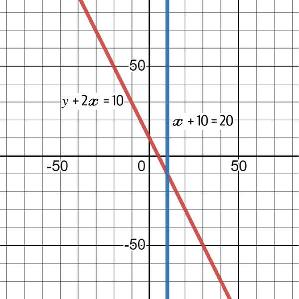
Figure 4-6. A graph showing the two functions and their intersection (solution)

As the functions are linear, solving them can result in one of three outcomes:

1. There is only one solution for each variable.
2. There is no solution. This occurs when the functions are parallel (this means that they never intersect).
3. There are an infinite number of solutions. This occurs when, through simplification, both functions are the same (since all points fall on the straight line).

Before moving on to solving systems of equations using algebra, let’s visually see how there can be no solution and how there can be an infinite number of solutions. Consider the following system:

$2x=10$

$4x=20$

Figure 4-7 charts the two together. Since they are exactly the same equation, they fall on the same line. In reality, there are two lines in Figure 4-7, but since they are the same, they are indistinguishable. For every x on the line, there is a corresponding y.

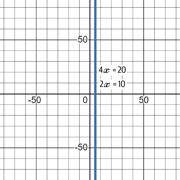
Figure 4-7. A graph showing the two functions and their infinite intersections

Now consider the following system:

$3x=10$

$6x=10$

Figure 4-8 shows how they never intersect, which is intuitive as you cannot multiply the same number (represented by the variable x) with different numbers and expect to get the same result.

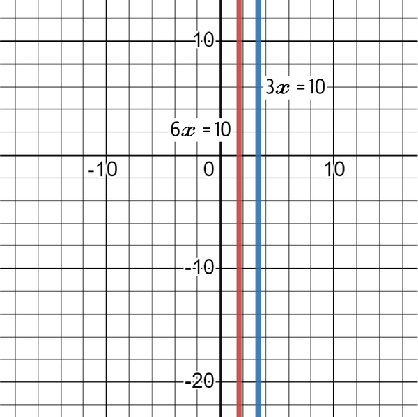
Figure 4-8. A graph showing the two functions and their impossible intersection

Algebraic methods are used when there are more than two variables since they cannot be solved through graphs. This mainly entails two methods: substitution and elimination.

Substitution is used when you can replace the value of a variable in one equation and plug it into the second equation. Consider the following example:

$x+y=2$

$10x+y=10$

The easiest method is to rearrange the first equation so that you have y in terms of x:

$y=2-x$

$10x+(2-x)=10$

Solving for x in the second equation becomes simple:

$\begin{array}{c}10x+(2-x)=10\hfill \\ 10x+2-x=10\hfill \\ 10x-x=10-2\hfill \\ 9x=8\hfill \\ x=\frac{8}{9}\hfill \\ x=0.8889\hfill \end{array}$

Now that you have found the value of x, you can easily find y by plugging the value of x into the first equation:

$\begin{array}{c}0.8889+y=2\hfill \\ y=2-0.8889\hfill \\ y=1.111\hfill \end{array}$

To check if your solution is correct, you can plug in the values of x and y in both formulas:

$\begin{array}{c}0.8889+1.111=2\hfill \\ (10\times 0.8889)+1.111=10\hfill \end{array}$

Graphically, this means that the two equations intersect at (0.8889, 1.111). This technique can be used with more than two variables. Follow the same process until the equations are simplified enough to give you the answers. The issue with substitution is that it may take some time when you’re dealing with more than two variables.

Elimination is a faster alternative. It is about eliminating variables until there is only one left. Consider the following example:

$\begin{array}{c}2x+4y=20\hfill \\ 3x+2y=10\hfill \end{array}$

Noticing that there is 4y and 2y, it is possible to multiply the second equation by 2 so that you can subtract the equations from each other (which will remove the y variable):

$\begin{array}{c}2x+4y=20\hfill \\ 6x+4y=20\hfill \end{array}$

Subtracting the two equations from each other gives the following result:

$\begin{array}{c}-4x=0\hfill \\ x=0\hfill \end{array}$

Therefore, x = 0. Graphically, this means that they intersect whenever x = 0 (exactly at the vertical y line). Plugging the value of x into the first formula gives y  = 5:

$\begin{array}{c}(2\times 0)+4y=20\hfill \\ 4y=20\hfill \\ y=5\hfill \end{array}$

Similarly, elimination can also solve equations with three variables. The choice between substitution and elimination depends on the type of equation being solved.

Note

The key takeaways from this section are as follows:

• Systems of equations solve variables together. They are very useful in machine learning and are used in some algorithms.
• Graphical solutions are preferred for simple systems of equations.
• Solving systems of equations through algebra entails the use of substitution and elimination methods.
• Substitution is preferred when the system is simple, but elimination is the way to go when the system is a bit more complex.

Trigonometry

Trigonometry explores the behavior of what is known as trigonometric functions that relate the angles of a triangle to the lengths of its sides. The most-used triangle is the right-angled triangle, which has one angle at 90°. Figure 4-9 shows an example of a right-angled triangle.

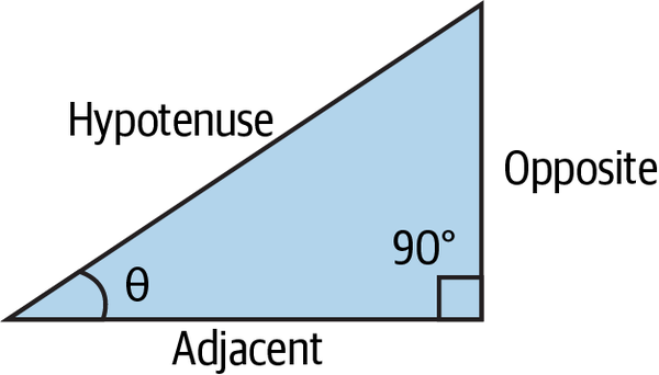
Figure 4-9. A right-angled triangle

Let’s define the main characteristics of a right-angled triangle:

• The longest side of the triangle is called the hypotenuse.
• The angle in front of the hypotenuse is the right angle (the one at 90°).
• Depending on the other angle (θ) you choose (from the two that remain), the line between this angle and the hypotenuse is called the adjacent and the other line is called the opposite.

Note

Trigonometric functions are mathematical functions used to relate the angles of a right triangle to the ratios of its sides. They have various applications in fields like geometry, physics, engineering, and more. They help analyze and solve problems related to angles, distances, oscillations, and waveforms, among other things.

Trigonometric functions are simply the division of one line by another line. Remember that you have three lines in a triangle (hypotenuse, opposite, and adjacent). The trigonometric functions are found as follow:

$sin\left(\theta \right)=\frac{\text{Opposite}}{\text{Hypotenuse}}$

$cos\left(\theta \right)=\frac{\text{Adjacent}}{\text{Hypotenuse}}$

$tan\left(\theta \right)=\frac{\text{Opposite}}{\text{Adjacent}}$

From the previous three trigonometric functions, it is possible to extract a trigonometric identity that reaches tan from sin and cos using basic linear algebra:

$tan\left(\theta \right)=\frac{sin\left(\theta \right)}{cos\left(\theta \right)}$

Hyperbolic functions are similar to trigonometric functions but are defined using exponential functions. Before understanding hyperbolic functions, one must understand Euler’s number.

Note

This part on hyperbolic functions is interesting as it forms the basis of what is known as activation functions, a key concept in neural networks, the protagonists of deep learning models. You will see them in detail in Chapter 8.

Euler’s number (denoted as e) is one of the most important numbers in mathematics. It is an irrational number, which is a real number that cannot be expressed as a fraction. The word irrational comes from the fact that there is no ratio to express it; it has nothing to do with its personality. Euler’s number is also the base of the natural logarithm ln, and the first digits of it are 2.71828. One of the best approximations to get e is the following formula:

$e={(1+\frac{1}{n})}^n$

By increasing n in the previous formula, you will approach the value of e. Euler’s number has many interesting properties, most notably the fact that its slope is its own value. Consider the following function (also called the natural exponent function):

$f\left(x\right)=e^x$

At any point, the slope of the function is the same value. Take a look at Figure 4-10.

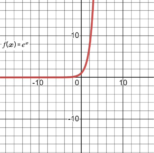
Figure 4-10. A graph of the natural exponent function

Note

You may be wondering why I am explaining exponents and logarithms in this book. There are mainly two reasons for this:

• Exponents and, more importantly, Euler’s number are used in hyperbolic functions where tanh(x) is one of the main activation functions for neural networks, a type of machine and deep learning model.
• Logarithms are useful in loss functions, a concept that you will see in later chapters.

Hyperbolic functions use the natural exponent function and are defined as follows:

$sinh\left(x\right)=\frac{e^x-e^{-x}}{2}$

$cosh\left(x\right)=\frac{e^x+e^{-x}}{2}$

$tanh\left(x\right)=\frac{e^x-e^{-x}}{e^x+e^{-x}}$

Among the key characteristics of tanh(x) are nonlinearity, the limitation between [–1, 1], and the fact that it is centered at zero. Figure 4-11 shows the graph of tanh(x).

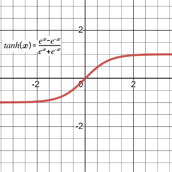
Figure 4-11. A graph of tanh(x) showing how it’s limited between –1 and 1

Note

The key takeaways from this section are as follows:

• Trigonometry is a field that explores the behavior of trigonometric functions that relate the angles of a triangle to the lengths of its sides.
• A trigonometric identity is a shortcut that relates the trigonometric functions with each other.
• Euler’s number e is irrational and is the base of the natural logarithm. It has many applications in exponential growth and in hyperbolic functions. 
• The hyperbolic tangent function is used in neural networks, a deep learning algorithm. 

Calculus

As previously mentioned, calculus is a branch of mathematics that focuses on the study of rates of change and accumulation of quantities. It consists of two primary branches: differential calculus (which deals with derivatives) and integral calculus (which deals with integration). This section briefly introduces both types of calculus while also discussing topics such as limits and optimization.

Limits and Continuity

Calculus works by making visible the infinitesimally small.

—Keith Devlin

Limits don’t have to be nightmarish. I have always found them to be misunderstood. They are actually quite easy to get. But first, you need motivation, and this comes from knowing the added value of learning limits.

Understanding limits is important in machine learning models for many reasons:

Optimization

In optimization methods like gradient descent, limits can be used to regulate the step size and guarantee convergence to a local minimum.

Feature selection

Limits can be used to rank the significance of various model features and perform feature selection, which can make the model simpler and perform better.

Sensitivity analysis

A machine learning model’s sensitivity to changes in input data and its capacity to generalize to new data can be used to examine a model’s behavior.

Also, limits are used in more advanced calculus concepts that you will learn about shortly.

The main aim of limits is to know the value of a function when it’s undefined. But what is an undefined function? When you have a function that gives a solution that is not possible (such as dividing by zero), limits help you bypass this issue in order to know the value of the function at that point. So the aim of limits is to solve functions even when they are undefined.

Remember that the solution to a function that takes x as an input is a value in the y-axis. Figure 4-12 shows a linear graph of the following function:

$f\left(x\right)=x+2$

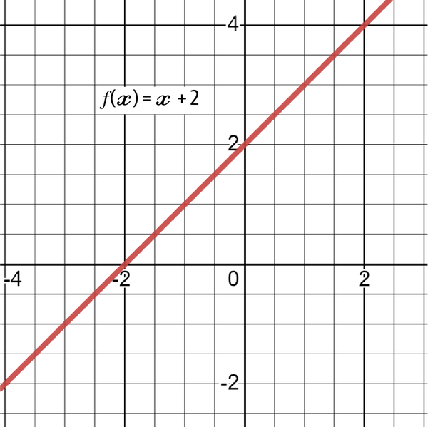
Figure 4-12. A graph of the function f(x) = x + 2

The solution of the function in the graph is the one that lies on the linear line taking into account the value of x every time.

What would be the solution of the function (the value of y) when x = 4? Clearly, the answer is 6, as substituting the value of x with 4 gives 6:

$f\left(4\right)=4+2=6$

Thinking of this solution in terms of limits would be like asking for the solution of the function as x approaches 4 from both sides (the negative/decreasing side and the positive/increasing side). Table 4-1 simplifies this dilemma.

Table 4-1. Finding x as it approaches 4

f(x)	x
5.998	3.998
5.999	3.999
6.000	4.000
6.001	4.001
6.002	4.002

Approaching from the negative side is the equivalent of adding a fraction of a number while below 4 and analyzing the result every time. Similarly, approaching from the positive side is the equivalent of removing a fraction of a number while above 4 and analyzing the result every time. The solution seems to converge to 6 as x approaches 4. This is the solution to the limit.

Limits in the general form are written following this convention:

${lim}_{x\to a}f\left(x\right)=L$

The general form of the limit is read as follows: as you approach a along the x-axis (whether from the positive or the negative side), the function f(x) gets closer to the value of L.

Note

The idea of the limit states that as you lock in and approach a number from either side (negative or positive), the solution of the equation approaches a certain number, and the solution to the limit is that number.

As mentioned previously, limits are useful when the exact point of the solution is undefined using the conventional way of substitution.

A one-sided limit is different from the general limit. With a lefthand limit, you search for the limit going from the negative side to the positive side, and with a righthand limit, you search for the limit going from the positive side to the negative side. The general limit exists when the two one-sided limits exist and are equal. Therefore, the previous statements are summarized as follows:

• The lefthand limit exists.
• The righthand limit exists.
• The lefthand limit is equal to the righthand limit.

The lefthand limit is defined as follows:

${lim}_{x\to a^{-}}f\left(x\right)=L$

The righthand limit is defined as follows:

${lim}_{x\to a^{+}}f\left(x\right)=L$

Consider the following equation:

$f\left(x\right)=\frac{x^3-27}{x-3}$

What is the solution of the function when x = 3? Substitution leads to the following issue:

$f\left(3\right)=\frac{3^3-27}{3-3}=\frac{27-27}{3-3}=\frac{0}{0}=\text{Undefined}$

However, thinking about this in terms of limits as shown in Table 4-2, it seems that as you approach x = 3, either from the left or right side, the solution tends to approach 27.

Table 4-2. Finding x as it approaches 3

f(x)	x
2.9998	26.9982
2.9999	26.9991
3.0000	Undefined
3.0001	27.0009
3.0002	27.0018

Graphically, this can be seen as a discontinuity in the chart along both axes. The discontinuity exists on the line around the coordinate (3, 27). Some functions do not have limits. For example, what is the limit of the following function as x approaches 5?

${lim}_{x\to 5}\frac{1}{x-5}$

Looking at Table 4-3, it seems that as x approaches 5, the results highly diverge when approaching from both sides. For instance, approaching from the negative side, the limit of 4.9999 is –10,000, and from the positive side, the limit of 5.0001 is 10,000.

Table 4-3. Finding x as it approaches 5

f(x)	x
4.9998	–5000
4.9999	–10000
5.0000	Undefined
5.0001	10000
5.0002	5000

Remember that for the general limit to exist, both one-sided limits must exist and must be equal, which is not the case here. Graphing this gives Figure 4-13, which may help you understand why the limit does not exist.

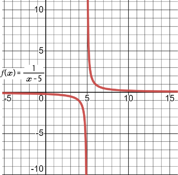
Figure 4-13. A graph of the function proving that the limit does not exist

But what if the function that you want to analyze looks like this:

${lim}_{x\to 5}\frac{1}{|x-5|}$

Looking at Table 4-3, it seems that as x approaches 5, the results rapidly accelerate as they diverge to a very big number referred to as infinity (∞):

$f\left(x\right)=\frac{1}{|x-5|}$

Take a look at Table 4-4:

Table 4-4. Another attempt at finding x as it approaches 5

f(x)	x
4.99997	334333.33
4.99998	50000
4.99999	100000
4.9999999	10000000
5.00000	Undefined
5.0000001	10000000
5.00001	100000
5.00002	50000
5.00003	334333.33

At every tiny step, x approaches 5, and y approaches positive infinity. The answer to the limit question is therefore positive infinity (+∞). Figure 4-14 shows the graph of the function. Notice how both sides rise in value as x approaches 5.

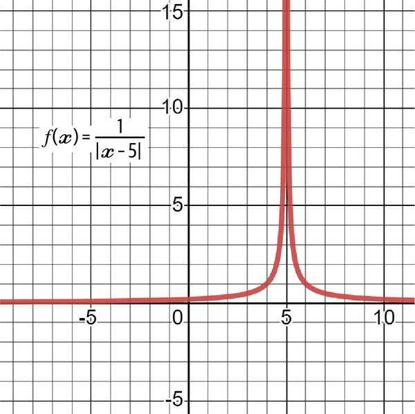
Figure 4-14. A graph of the function proving that the limit exists as x approaches 5

To Infinity and Beyond

You can understand what infinity represents in terms of mathematics. Infinity is an idea or a concept rather than a number. The symbol (∞) is often referred to as a lemniscate.

Positive infinity (∞) and negative infinity (–∞) are both concepts that exist across the axis where the former tends toward the right and the latter tends toward the left.

Interestingly, infinity is often thought of as an ever-growing measure, but it is not expanding or getting bigger. It is already what it is.

Mathematical operations, including the concept of infinity, may be hard to grasp and have many considerations. One of the most interesting examples is the answer to why the result of 1 divided by zero is undefined.

Imagine dividing an apple among 10 people; normally every person will get an equal fraction (1/10) of that apple until the apple is consumed. But what if you want to divide the apple by zero people? The number of people required to consume the apple will tend toward infinity (the logic is hard to grasp, but mathematically you can think of infinitesimally small parts of the apple requiring a huge number of people to consume them).

Therefore, following this logic, you can say that 1 divided by 0 is infinity and is actually defined. So, why is it generally considered undefined? The issue is that the apple example describes positive infinity, and if you want to follow the example of dividing 1 by infinitesimally small negative numbers that tend toward zero, then you will also say that 1 divided by 0 is negative infinity.

So which is it? Positive or negative infinity? Because of this conflict, the result is undefined.

Continuous functions are ones that are drawn without gaps or holes in the graph, while discontinuous functions contain such gaps and holes. This usually means that the latter contain points where the solution of the functions is undefined and may need to be approximated by limits. Therefore, continuity and limits are two related concepts.

Let’s proceed to solving limits; after all, you are not going to create a table every time and analyze the results subjectively to find the limits. There are three ways to solve limits:

• Substitution: This is the simplest rule and is generally used first.
• Factoring: This comes after substitution does not work.
• Conjugate methods: This solution comes after the first two do not work.

Substitution involves simply plugging in the value that x approaches. Basically, these are functions that have solutions where the limits are used. Take the following example:

${lim}_{x\to 5}x+10-2x$

Using substitution, the limit of the function is found as follows:

$\begin{array}{c}\hfill \underset{x\to 5}{lim}x+10-2x=5+10-(2\times 5)=5\end{array}$

Therefore, the answer to the limit is 5.

Factoring is the next option when substitution does not work (e.g., the limit is undefined after plugging the value of x into the function). Factoring is all about changing the form of the equation using factors in such a way that the equation is not undefined anymore when using substitution. Take the following example:

${lim}_{x\to -6}\frac{(x+6)(x^2-x+1)}{x+6}$

If you try substitution, you will get an undefined value as follows:

$\begin{array}{c}\hfill \underset{x\to -6}{lim}\frac{(x+6)(x^2-x+1)}{x+6}=\frac{(-6+6)({(-6)}^2-(-6)+1)}{-6+6}=\frac{0}{0}=\text{Undefined}\end{array}$

Factoring may help in this case. For example, the nominator is multiplied by (x + 6) and then divided by (x + 6). Simplifying this by canceling the two terms could give a solution:

${lim}_{x\to -6}\frac{(x+6)(x^2-x+1)}{x+6}={lim}_{x\to -6}{x}^2-x+1$

Now that factoring is done, you can try substitution once again:

${lim}_{x\to -6}{x}^2-x+1={(-6)}^2-(-6)+1=43$

The limit of the function as x tends toward –6 is therefore 43.

Forming a conjugate is the next option when substitution and factoring do not work. A conjugate is formed by simply changing signs between two variables. For example, the conjugate of x + y is  x – y. The way to do this in the case of a fraction is to multiply the nominator and the denominator by the conjugate of one of them (with a preference to use the conjugate of the term that has a square root since it will get canceled out). Consider the following example:

${lim}_{x\to 9}\frac{x-9}{\sqrt{x}-3}$

By multiplying both terms by the conjugate of the denominator, you will have started to use the conjugate method to solve the problem:

${lim}_{x\to 9}\frac{x-9}{\sqrt{x}-3}\left(\frac{\sqrt{x}+3}{\sqrt{x}+3}\right)$

Taking into account the multiplication and then simplifying gives the following:

${lim}_{x\to 9}\frac{(x-9)(\sqrt{x}+3)}{(\sqrt{x}-3)(\sqrt{x}+3)}$

You will be left with the following familiar situation:

${lim}_{x\to 9}\frac{(x-9)(\sqrt{x}+3)}{x-9}$

${lim}_{x\to 9}\sqrt{x}+3$

Now the function is ready for substitution:

${lim}_{x\to 9}\sqrt{9}+3=3+3=6$

The solution to the function is therefore 6. As you can see, sometimes work needs to be done on the equations before they are ready for substitution.

Note

The key takeaways from this section are as follows:

• Limits help find solutions for functions that may be undefined in certain points.
• For the general limit to exist, the two one-sided limits must exist and must be equal.
• There are ways to find the limit of a function, notably substitution, factoring, and forming the conjugate.

Derivatives

A derivative measures the change in a function given a change of one or more of its inputs. In other words, it is the rate of change of a function at a given point.

Having a solid understanding of derivatives is important in building machine learning models, for multiple reasons:

Optimization

To minimize the loss function, optimization methods employ derivatives to ascertain the direction of the steepest descent and modify the model’s parameters.

Backpropagation

To execute gradient descent in deep learning, the backpropagation technique uses derivatives to calculate the gradients of the loss function with respect to the model’s parameters.

Hyperparameter tuning

To improve the performance of the model, derivatives are used for sensitivity analysis and tuning of hyperparameters.

Do not forget what you learned from the previous section on limits, as you will need this knowledge for this section as well. Calculus mainly deals with derivatives and integrals. This section discusses derivatives and their uses.

You can consider derivatives to be functions that represent (or model) the slope of another function at some point. A slope is a measure of a line’s position relative to a horizontal line. A positive slope indicates a line moving up, while a negative slope indicates a line moving down.

Derivatives and slopes are related concepts, but they are not the same thing. Here’s the main difference between the two:

Slope

The slope measures the steepness of a line. It is the ratio of the change in the y-axis to the change in the x-axis.

Derivative

The derivative describes the rate of change of a given function. As the distance between two points on a function approaches zero, the derivative of that function at that point is the limit of the slope of the tangent line.

Before explaining derivatives in layperson’s terms and showing some examples, let’s see their formal definitions:

$f^{\text{'}}\left(x\right)={lim}_{h\to 0}\frac{f(x+h)-f\left(x\right)}{h}$

The equation forms the basis of solving derivatives, although there are many shortcuts that you will learn about. Let’s try finding the derivative of a function using the formal definition. Consider the following equation:

$f\left(x\right)=x^2+4x-2$

To find the derivative, plug f(x) into the formal definition and then solve the limit:

$f^{\text{'}}\left(x\right)={lim}_{h\to 0}\frac{f(x+h)-f\left(x\right)}{h}$

To simplify things, let’s find f(x + h) so that plugging it into the formal definition becomes easier:

$f(x+h)={(x+h)}^2+4(x+h)-2$

$f(x+h)=x^2+2xh+h^2+4x+4h-2$

Now let’s plug f(x + h) into the definition:

$f^{\text{'}}\left(x\right)={lim}_{h\to 0}\frac{x^2+2xh+h^2+4x+4h-2-x^2-4x+2}{h}$

Notice how there are many terms that can be simplified so that the formula becomes clearer. Remember, you are trying to find the limit for the moment, and the derivative is found after solving the limit:

$f^{\text{'}}\left(x\right)={lim}_{h\to 0}\frac{2xh+h^2+4h}{h}$

The division by h gives further potential for simplification since you can divide all the terms in the numerator by the denominator h:

$f^{\text{'}}\left(x\right)={lim}_{h\to 0}2x+h+4$

It’s now time to solve the limit. Because the equation is simple, the first attempt is by substitution, which, as you have guessed, is possible. By substituting the variable h and making it zero (according to the limit), you are left with the following:

$f^{\text{'}}\left(x\right)=2x+4$

That is the derivative of the original function f(x). If you want to find the derivative of the function when x = 2, you simply have to plug 2 into the derivative function:

$f^{\text{'}}\left(2\right)=2\left(2\right)+4=8$

Figure 4-15 shows the original function’s graph with the derivative (the straight line). Notice how f'(2) lies exactly at 8. The slope of f(x) when x = 2 is 8.

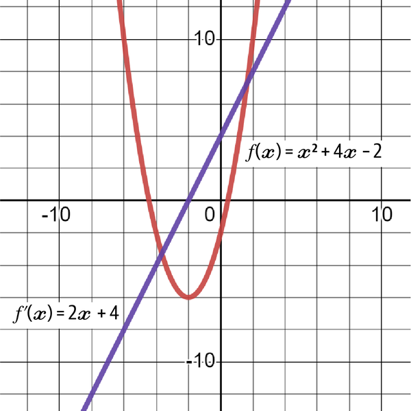
Figure 4-15. The original f(x) with its derivative f'(x)

Note

Notice that when f(x) hits the bottom and starts rising, f'(x) crosses the zero line.

You are unlikely to use the formal definition every time you want to find a derivative. There are derivative rules that allow you to save a lot of time through shortcuts. The first rule is referred to as the power rule, which is a way to find the derivative of functions with exponents.

It is common to also refer to derivatives using this notation (which is the same thing as f'(x)):

$\frac{dy}{dx}$

The power rule for finding derivatives is as follows:

$\frac{dy}{dx}\left(a{x}^n\right)=(a.n)x^{n-1}$

Basically, this means that the derivative is found by multiplying the constant by the exponent and then subtracting 1 from the exponent. Here’s an example:

$f\left(x\right)=x^4$

$f^{\text{'}}\left(x\right)=(1\times 4)x^{(4-1)}=4x^3$

Remember that if there is no constant attached to the variable, it means that the constant is equal to 1. Here’s a more complex example with the same principle:

$f\left(x\right)=2x^2+3x^7-2x^3$

$f^{\text{'}}\left(x\right)=4x+21x^6-6x^2$

It is worth noting that the rule also applies to constants even though they do not satisfy the general form of the power rule. The derivative of a constant is zero. While it helps to know why, first you must be aware of the following mathematical concept:

$x^0=1$

That being said, you can imagine constants as always being multiplied by x to the power of zero (since doing so does not change their value). Now, if you want to find the derivative of 17, here’s how it would go:

$17=17x^0=(0\times 17)x^{0-1}=0x^{-1}=0$

As you know, anything multiplied by zero returns zero as a result. This gives the constants rule for derivatives as follows:

$\frac{dy}{dx}\left(a\right)=0$

You follow the same logic when encountering fractions or negative numbers in the exponents.

The product rule of derivatives is useful when there are two functions multiplied by each other. The product rule is as follows:

$\frac{dy}{dx}\left[f\left(x\right)g\left(x\right)\right]=f^{\text{'}}\left(x\right)g\left(x\right)+f\left(x\right)g^{\text{'}}\left(x\right)$

Let’s take an example and find the derivative using the product rule:

$h\left(x\right)=(x^2+2)(x^3+1)$

The equation can clearly be segmented into two terms, f(x) and g(x), like this:

$f\left(x\right)=(x^2+2)$

$g\left(x\right)=(x^3+1)$

Let’s find the derivatives of the two terms before applying the product rule. Notice that finding the derivative of f(x) and g(x) is easy once you understand the power rule:

$f^{\text{'}}\left(x\right)=2x$

$g^{\text{'}}\left(x\right)=3x^2$

When applying the product rule, you should get the following:

$h^{\text{'}}\left(x\right)=(x^2+2)\left(3x^2\right)+\left(2x\right)(x^3+1)$

$h^{\text{'}}\left(x\right)=3x^4+6x^2+2x^4+2x$

$h^{\text{'}}\left(x\right)=5x^4+6x^2+2x$

Figure 4-16 shows the graph of h(x) and h'(x).

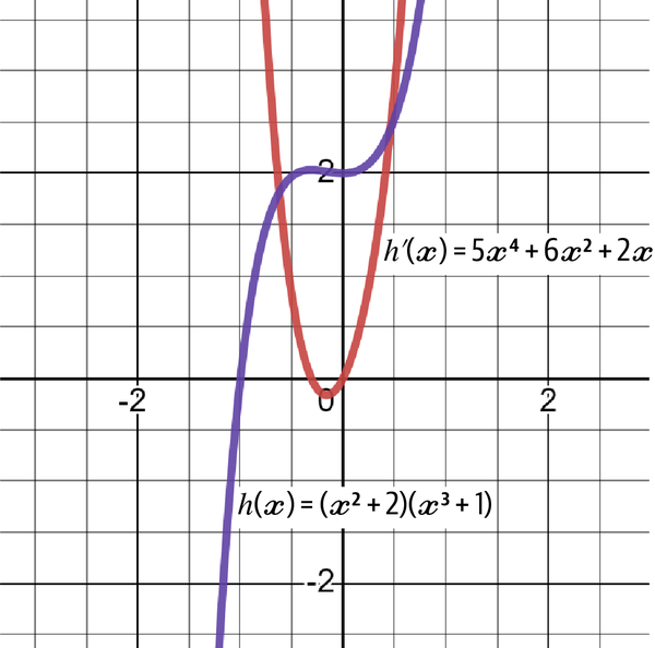
Figure 4-16. The original h(x) with its derivative h'(x)

Now let’s turn our attention to the quotient rule, which deals with the division of two functions. The formal definition is as follows:

$\frac{dy}{dx}\left[\frac{f\left(x\right)}{g\left(x\right)}\right]=\frac{f^{\text{'}}\left(x\right)g\left(x\right)-f\left(x\right)g^{\text{'}}\left(x\right)}{{\left[g\left(x\right)\right]}^2}$

Let’s apply it to the following function:

$f\left(x\right)=\frac{x^2-x+1}{x^2+1}$

As usual, it’s better to start by finding the derivatives of f(x) and g(x), which in this case are clearly separated, with f(x) being the nominator and g(x) being the denominator. When applying the quotient rule, you should get the following:

$f^{\text{'}}\left(x\right)=\frac{(2x-1)(x^2+1)-(x^2-x+1)\left(2x\right)}{{(x^2+1)}^2}$

$f^{\text{'}}\left(x\right)=\frac{2x^3+2x-x^2-1-2x^3+2x^2-2x}{{(x^2+1)}^2}$

$f^{\text{'}}\left(x\right)=\frac{x^2-1}{{(x^2+1)}^2}$

Exponential derivatives deal with the power rule applied to constants. Take a look at the following equation. How would you find its derivative?

$f\left(x\right)=a^x$

Instead of the usual variable-base-constant-exponent, it is constant-base-variable-exponent. This is treated differently when trying to calculate the derivative. The formal definition is as follows:

$\frac{dy}{dx}{a}^x=a^x(lna)$

The following example shows how this is done:

$\frac{dy}{dx}{4}^x=4^x(ln4)$

Euler’s number, mentioned earlier, has a special derivative. When it comes to finding the derivative of e, the answer is interesting:

$\frac{dy}{dx}{e}^x=e^x(lne)=e^x$

This is because the natural log function and the exponential function are inverses of each other, so the term ln e equals 1. Therefore, the derivative of the exponential function e is itself.

In parallel, let’s discuss logarithmic derivatives. By now, you should know what exponents and logarithms are. The general definition for both types of logarithms is as follows:

$\frac{dy}{dx}{log}_{a}x=\frac{1}{xlna}$

$\frac{dy}{dx}lnx={log}_{e}x=\frac{1}{xlne}=\frac{1}{x}$

Notice how in the second derivative function of the natural logarithm, the term ln e is once again encountered, thus making simplification quite easy since it is equal to 1.

Take the following example:

$f\left(x\right)=7lo{g}_2\left(x\right)$

Using the formal definition, the derivative of this logarithmic function is as follows:

$f^{\text{'}}\left(x\right)=7\left(\frac{1}{xln2}\right)=\frac{7}{xln2}$

Note

The logarithm log has a base of 10, but the natural logarithm ln has a base of e (~2.7182).

The natural logarithm and the log function are actually linearly related through simple multiplication. If you know the log of the constant a, you can find its natural logarithm ln by multiplying the log of a by 2.4303.

One major concept in derivatives is the chain rule. Let’s back up to the power rule, which deals with exponents on variables. Remember the following formula to find the derivative:

$\frac{dy}{dx}\left(a{x}^n\right)=(a.n)x^{n-1}$

This is a simplified version because there is only x, but the reality is that you must multiply by the derivative of the term under the exponent. Until now, you have seen only x as the variable under the exponent. The derivative of x is 1, which is why it is simplified and rendered invisible. However, with more complex functions such as this one:

$f\left(x\right)={(4x+1)}^2$

The derivative of the function is found by following these two steps:

1. Find the derivative of the outside function without touching the inside function.
2. Find the derivative of the inside function and multiply it by the rest of the function.

The solution is therefore as follows (knowing that the derivative of 4x + 1 is just 4):

$f^{\text{'}}\left(x\right)=2(4x+1).4$

$f^{\text{'}}\left(x\right)=8(4x+1)$

$f^{\text{'}}\left(x\right)=32x+8$

The same applies with the exponential functions. Take the following example:

$f\left(x\right)=e^x$

$f^{\text{'}}\left(x\right)=e^x\left(1\right)=e^x$

The chain rule can actually be considered a master rule as it applies anywhere, even in the product rule and the quotient rule.

There are more concepts to master in derivatives, but as this book is not meant to be a full calculus master class, you should at least know the meaning of a derivative, how it is found, what it represents, and how it can be used in machine and deep learning.

Note

The key takeaways from this section are as follows:

• A derivative measures the change in a function given a change of one or more of its inputs.
• The power rule is used to find the derivative of a function raised to a power.
• The product rule is used to find the derivative of two functions that are multiplied together.
• The quotient rule is used to find the derivative of two functions that are divided by each other.
• The chain rule is the main rule used in differentiating (which means the process of finding the derivative). Due to simplicity, it is often overlooked.
• Derivatives play a crucial role in machine learning, such as enabling optimization techniques, aiding model training, and enhancing the interpretability of the models.

Integrals and the Fundamental Theorem of Calculus

An integral is an operation that represents the area under a curve of a function given an interval. It is the inverse of a derivative, which is why it is also called an antiderivative.

The process of finding integrals is called integration. Integrals can be used to find areas below a curve, and they are heavily used in the world of finance in such areas as risk management, portfolio management, probabilistic methods, and even option pricing.

The easiest way to understand an integral is to think of calculating an area below the curve of a function. This can be done by manually calculating the different changes in the x-axis, but adding these slices to find the area is a tedious process. This is where integrals come to the rescue.

Keep in mind that an integral is the inverse of a derivative. This is important because it implies a direct relationship between the two. The basic definition of an integral is as follows:

$\int f\left(x\right)dx=F\left(X\right)+C$

$\text{The}\int \text{symbol}\text{represents}\text{the}\text{integration}\text{process}$

$f\left(x\right)\text{is}\text{the}\text{derivative}\text{of}\text{the}\text{general}\text{function}F\left(x\right)$

$C\text{represents}\text{the}\text{lost}\text{constant}\text{in}\text{the}\text{differentiation}\text{process}$

$dx\text{represents}\text{slicing}\text{along}x\text{as}\text{it}\text{approaches}\text{zero}$

The preceding equation means that the integral of f(x) is the general function F(x) plus a constant C, which was lost in the initial differentiation process. Here’s an example to better explain the need to put in the constant.

Consider the following function:

$f\left(x\right)=x^2+5$

Calculating its derivative, you get the following result:

$f^{\text{'}}\left(x\right)=2x$

Now, what if you wanted to integrate it so that you go back to the original function (which in this case is represented by the capital letter F(x) instead of f(x))?

$\int 2xdx$

Normally, having seen the differentiation process (which means taking the derivative), you would return 2 as the exponent, which gives you the following answer:

$\int 2xdx=x^2$

This does not look like the original function. It’s missing the constant 5. But you have no way of knowing that, and even if you knew there was a constant, you would have no way of knowing what it is: 1? 2? 677? This is why a constant C is added in the integration process to represent the lost constant. Therefore, the answer to the integration problem is as follows:

$\int 2xdx=x^2+C$

Note

Up until now, the discussion has been limited to indefinite integrals where the integration symbol is naked (which means there are no boundaries to it). You will see what this means right after we define the necessary rules to complete the integration.

For the power function (just like the previous function), the general rule for integration is as follows:

$\int x^{a}dx=\frac{x^{a+1}}{a+1}+C$

This is much simpler than it looks. You are just reversing the power rule you saw earlier. Consider the following example:

$\int 2x^{6}dx$

$\int 2x^{6}dx=\frac{2x^7}{7}+C$

$\int 2x^{6}dx=\frac{2}{7}{x}^7+C$

To verify your answer, you can find the derivative of the result (using the power rule):

$F\left(x\right)=\frac{2}{7}{x}^7+C$

$f^{\text{'}}\left(x\right)=\left(7\right)\frac{2}{7}{x}^{7-1}+0$

$f^{\text{'}}\left(x\right)=2x^6$

Let’s take another example. Consider the following integration problem:

$\int 2dx$

Naturally, using the rule, you should find the following result:

$\int 2dx=2x+C$

Let’s move on to definite integrals, which are integrals with numbers on the top and bottom that represent intervals below a curve of a function. Hence, indefinite integrals find the area under the curve everywhere, and definite integrals are bounded within an interval given by point a and point b. The general definition of indefinite integrals is as follows:

${\int }_a^{b}f\left(x\right)dx=F\left(B\right)-F\left(A\right)$

This is as simple as it gets. You will solve the integral, then plug in the two numbers and subtract the two functions from each other. Consider the following evaluation of an integral (integral solving is commonly referred to as evaluating the integral):

${\int }_0^{6}3x^2-10x+4dx$

The first step is to understand what is being asked. From the definition of integrals, it seems that the area between [0, 2] on the x-axis is to be calculated using the given function:

$F\left(x\right)=\left([x^3-5x^2+4x+C]\right){|}_0^6$

To evaluate the integral at the given points, simply plug in the values as follows:

$F\left(x\right)=\left([6^3-5{\left(6\right)}^2+4\left(6\right)+C]\right)-\left([0^3-5{\left(0\right)}^2+4\left(0\right)+C]\right)$

$F\left(x\right)=\left(\right[216-180+24+C\left]\right)-\left(\right[0-0+0+C\left]\right)$

$F\left(x\right)=\left(\right[60+C\left]\right)-\left(\right[0+C\left]\right)$

$F\left(x\right)=(60-0)$

$F\left(x\right)=60$

Note

The constant C will always cancel out indefinite integrals, so you can leave it out in this kind of problem.

Therefore, the area below the graph of f(x) and above the x-axis, as well as between [0, 6] on the x-axis, is equal to 60 square units. The following shows a few rules of thumb on integrals (after all, this chapter is supposed to refresh your knowledge or give you a basic understanding of a few key mathematical concepts):

• To find the integral of a constant:

  $\int adx=ax+C$

• To find the integral of a variable:

  $\int xdx=\frac{1}{2}{x}^2+C$

• To find the integral of a reciprocal:

  $\int \frac{1}{x}dx=ln\left|x\right|+C$

• To find the integral of an exponential:

  $\int a^{x}dx=\frac{a^x}{ln\left(a\right)}+C$

  $\int e^{x}dx=e^x+C$

The fundamental theorem of calculus links derivatives with integrals. This means that it defines derivatives in terms of integrals and vice versa. The fundamental theorem of calculus is actually made up of two parts:

Part I

The first part of the fundamental theorem of calculus states that if you have a continuous function f(x), then the original function F(x) defined as the antiderivative of f(x) from a fixed starting point a up to x is a function that is differentiable everywhere from a to x, and its derivative is simply f(x) evaluated at x.

Part II

The second part of the fundamental theorem of calculus states that if you have a function f(x) that is continuous over a certain interval [a, b], and you define a new function F(x) as the integral of f(x) from a to x, then the definite integral of f(x) over that same interval [a, b] can be calculated as F(b) – F(a).

The theorem is useful in many fields, including physics and engineering, but optimization and other mathematical models also benefit from it. Some examples of using integrals in the different learning algorithms can be summed up as follows:

Density estimation

Integrals are used in density estimation, a part of many machine learning algorithms, to calculate the probability density function.

Reinforcement learning

Integrals are used in reinforcement learning to calculate expected values of reward functions. Reinforcement learning is covered in Chapter 10.

Note

The key takeaways from this section are as follows:

• Integrals are also known as antiderivatives and they are the opposite of derivatives.
• Indefinite integrals find the area under the curve everywhere, while definite integrals are bounded within an interval given by point a and point b.
• The fundamental theorem of calculus is the bridge between derivatives and integrals.
• In machine learning integrals are used for modeling uncertainty, making predictions, and estimating expected values.

Optimization

Several machine and deep learning algorithms depend on optimization techniques to decrease error functions.

Optimization is the process of finding the best solution among all possible solutions. Optimization is all about finding the highest and lowest points of a function. Figure 4-17 shows the graph for the following formula:

$f\left(x\right)=x^4-2x^2+x$

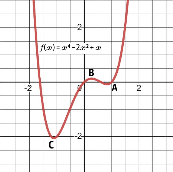
Figure 4-17. A graph of the function $f\left(x\right)=x^4-2x^2+x$

A local minimum exists when values on the right of the x-axis are decreasing until reaching a point where they start increasing. The point does not have to necessarily be the lowest point in the function, hence the name local. In Figure 4-17, the function has a local minimum at point A.

A local maximum exists when values on the right of the x-axis are increasing until reaching a point where they start decreasing. The point does not have to necessarily be the highest point in the function. In Figure 4-17, the function has a local maximum at point B.

A global minimum exists when values on the right of the x-axis are decreasing until reaching a point where they start increasing. The point must be the lowest point in the function, hence the name global. In Figure 4-17, the function has a global minimum at point C.

A global maximum exists when values on the right of the x-axis are increasing until reaching a point where they start decreasing. The point must be the highest point in the function. In Figure 4-17, there is no global maximum, as the function will continue infinitely without creating a top. You can clearly see how the function accelerates upward.

When dealing with machine and deep learning models, the aim is to find model parameters (or inputs) that minimize what is known as a loss function (a function that gives the error of forecasts). If the loss function is convex, optimization techniques should find the parameters that tend toward the global minimum where the loss function is minimized.

If the loss function is nonconvex, the convergence is not guaranteed, and the optimization may only lead toward approaching a local minimum, which is a part of the aim, but this leaves the global minimum, which is the final aim.

But how are these minima and maxima found? Let’s look at it step by step:

1. The first step is to perform the first derivative test (which is calculating the derivative of the function). Then, setting the function equal to zero and solving for x will give what are known as critical points. Critical points are the points where the function changes direction (the values stop going in one direction and start going in another direction). Therefore, these points are maxima and minima.
2. The second step is to perform the second derivative test (which is simply calculating the derivative of the derivative). Then, setting the function equal to zero and solving for x will give what are known as inflection points. Inflection points show where the function is concave up and where it is concave down.

In other words, critical points are where the function changes direction, and inflection points are where the function changes concavity. Figure 4-18 shows the difference between a concave up function and a concave down function.

$\text{Concave}\text{up}\text{function}=x^2$

$\text{Concave}\text{down}\text{function}=-x^2$

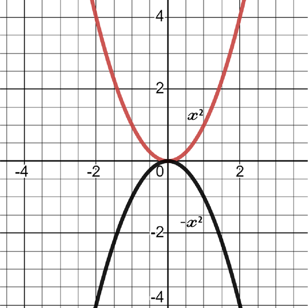
Figure 4-18. A concave up function and a concave down function

The steps to find the extrema are as follows:

1. Find the first derivative and set it to zero.
2. Solve the first derivative to find x. The values are called critical points, and they represent the points where the function changes direction.
3. Plug values into the formula that are either below or above the critical points. If the result of the first derivative is positive, it means that it’s increasing around that point, and if it’s negative, it means that it’s decreasing around that point.
4. Find the second derivative and set it to zero.
5. Solve the second derivative to find x. The values, called inflection points, represent the points where concavity changes from up to down and vice versa.
6. Plug values into the formula that are either below or above the inflection points. If the result of the second derivative is positive, it means there is a minimum at that point, and if it’s negative, it means there is a maximum at that point.

It is important to understand that the first derivative test relates to critical points and the second derivative test relates to inflection points. The following example finds the extrema of the function:

$f\left(x\right)=x^2+x+4$

The first step is to take the first derivative, set it to zero, and solve for x:

$f^{\text{'}}\left(x\right)=2x+1$

$2x+1=0$

$x=-\frac{1}{2}$

The result shows there is a critical point at that value. Now find the second derivative:

$f^{\text{'}\text{'}}\left(x\right)=2$

Next, the critical point must be plugged into the second derivative formula:

$f^{\text{'}\text{'}}(-\frac{1}{2})=2$

The second derivative is positive at the critical point. This means that there is a local minimum at that point.

In the coming chapters, you will see more complex optimization techniques such as the gradient descent and the stochastic gradient descent, which are fairly common in machine learning algorithms. Note that you do not have to fully understand the details of optimization and solving for the unknown variables as the algorithms will do that on their own.

Note

The key takeaways from this section are as follows:

• Optimization is the process of finding the function’s extrema.
• Critical points are the points where the function changes direction. 
• Inflection points give where the function is concave up and where it is concave down.
• A loss function is a function that measures the error of forecasts in predictive machine learning.

Summary

Chapters 2, 3, and 4 presented the main numerical concepts to help you start understanding basic machine and deep learning models. I made all reasonable efforts to simplify the technical details as much as possible. However, I encourage you to read these three chapters at least twice so that everything you have learned becomes second nature. I also encourage you to research these concepts in more depth in other material.

Naturally, deep learning requires more in-depth knowledge in mathematics, but I believe that with the concepts in this chapter, you may start dipping your toes into creating algorithms. After all, they come prebuilt from packages and libraries, and the aim of this chapter was to help you understand what you are working with. It is unlikely that you will build the models from scratch using archaic tools.

By now, you should have gained a certain understanding of data science and the mathematical requirements that will get you started comfortably. We have two more topics to cover before you can start building your first machine learning model: technical analysis and Python for data science.

¹ Matrices can also contain symbols and expressions, but for the sake of simplicity, let’s stick to numbers.