Data Modeling with Microsoft Power BI

Chapter 1. What Is a Data Model?

This chapter covers the basics of data modeling, starting with basic terms, which will help establish the reasoning behind taking so much care of the data model. A data model that is optimized for creating reports and doing analysis is much easier to work with than one that is optimized for other purposes (e.g., to store data for an application or data collected in a spreadsheet). When it comes to analytical databases and data warehouses, you have more than one option.

The goal throughout this book is to create the data model as a star schema. By the end of this chapter, you’ll know which characteristics of a star schema differentiate it from other modeling approaches. Each and every chapter reinforces why a star schema is so important when it comes to analytical databases in general and Power BI and Analysis Services tabular in particular. You will learn how to transform any data model into a star schema.

Transforming information of your data source(s) into a star schema is usually not an easy task. Quite the opposite; it can be difficult. It might take several iterations. It might take discussions with the people who you build the data model for—and the people using the reports, as well as those who are responsible for the data sources. You might face doubts (from others and yourself) about whether it’s really worth all the effort instead of avoiding the struggle and pulling the data in as it is. At such a point, it’s important to take a deep breath and evaluate whether a transformation would make the report creator’s life easier. If so, then it’s worth the effort. Repeat the data modeler’s mantra with me: make the report creator’s life easier.

Before I talk about transformations, I’ll introduce some basic terms and concepts:

• What is a data model?

• What is an entity? What does an entity have to do with a table?

• Why should you care about relationships?

• Why do you need to identify different keys (primary, foreign, and surrogate) and understand the general meaning of cardinality?

• How can you combine tables (set operators and joins)?

• What are the data modeling options?

The first stop on our journey toward the star schema is learning what a data model is in general terms.

Data Model

A model is something that represents the real world. It does not replicate it. Think of a map. A map replicating the real world 1:1 would be impractical: it would cover the whole planet. Instead, maps scale down distances. Maps are created for special purposes. A hiking map contains (and omits) different types of information than a road map does, and a nautical chart looks completely different still. All of these are maps but with different purposes.

The same applies to a data model, which represents a certain business logic. As with a map, a data model will look different for different use cases. Therefore, models for different industries will not be the same. And even organizations within the same industry will need different data models (even for basically identical business processes), as they will concentrate on different requirements. The challenges and solutions in this book will help you overcome obstacles when you build a data model for your organization.

Now for the bad news: there isn’t one data model that rules them all. Also, it’s impossible to create a useful data model with technical knowledge and no domain knowledge. But there is good news: this book will guide you through the technical knowledge necessary to successfully build data models for Power BI and/or Analysis Services tabular.

Don’t forget to collect or record all requirements from the business before creating the data model. Here are some examples of requirements in natural language:

• We sell goods to customers and need to know the day and the SKU of the product we sold

• We need to analyze the 12-month rolling average of the sold quantity for each product

• Up to 10 employees form a project team and we need to report the working hours per project task

These requirements will help you determine what information you need to store in which combinations and at which level of detail. There might be more than one option for the design of a data model for a certain use case.

And, very importantly, you need the create the correct data model right from the beginning. As soon as the first reports are created on a data model, every change in the model bears the risk of breaking those reports. The later you discover inconsistences and mistakes in your data model, the more expensive it will be to correct them. This cost hits everybody who created those reports—you yourself, but also other users who built reports based upon your data model.

The data model’s design has a huge impact on the performance of your reports, which query data from the data model to feed the visualizations as well. A well-designed data model lessens the need for query tuning later. And a well-designed data model can be used intuitively by the report creators, saving them time and effort (and saving your organization money). From a different point of view, problems with the performance of a report or report creators who are unsure of which tables and columns to use to gain certain insights are a sure sign of a data model that can be improved by a better choice of design.

In “Entity Relationship Diagrams”, I describe graphical ways to document a data model’s shape. But first, let’s discuss the entities of a data model.

Basic Components

You need to understand a few key components of a data model before you dive in. In this section, I explain the basic parts of a data model. In “Combining Tables”, I will walk you through different ways of combining tables with the help of set operators and joins and which kind of problems you can face and how to solve them.

Remember that this part of the book isn’t specific to Power BI. Some concepts may apply only when you prepare data before you connect Power Query to it (e.g., when writing a SQL statement in a relational database).

Entity

An entity is someone or something that can be individually identified. In natural language, entities are nouns. Think of a real person (your favorite teacher, for example), a product you bought recently (ice cream, anybody?), or a term (e.g., entity).

Entities can be both real and fictitious. And most have attributes: a name, value, category, point in time of creation, etc. These attributes are the information we are after when it comes to data. Attributes are displayed in reports to help the reader provide context, gain insights, and make decisions. They are used to filter displayed information to narrow down an analysis, too.

How do such entities make it into a data model? They’re stored in tables.

Tables

Tables are the base of a data model. They have been part of data models since at least 1970, when Edgar F. Codd developed the relational data model for his employer, IBM. But collecting information as lists or tables was done way before the invention of computers, as you can see when looking at old books.

Tables host entities: every entity is represented by a row in a table. Every attribute of an entity is represented by a column in a table. A column in a table has a name (e.g., birthday) and a data type (e.g., date). All rows of a single column must conform to this data type (it isn’t possible to store the place of birth in the column “birthday” for any row, for example). This is an important difference between a (database’s) table and a spreadsheet’s worksheet (e.g., in Excel). A single column in a single table contains content. You can see an example in Table 1-1.

Table 1-1. A table containing the name of doctors

Doctor’s name	Hire date
Smith	1993-06-03
Grey	2005-03-27
Young	2004-12-01
Stevens	2000-06-07
Karev	1998-09-19
O’Malley	2003-02-14

Entities do not exist just on their own but are related to each other.

Relationships

In most cases, relationships connect only two entities. In natural language, the relationship is represented by a verb (e.g., bought). Between the same two entities, more than one single relationship might exist. For example, a customer might have first ordered a certain product, which we later shipped. It’s the same customer and the same product but different relationships (ordered versus shipped).

Some relationships can be self-referencing. That means that there can be a relationship between one entity (one row in this table) and another entity of the same type (a different row in the same table). Organizational hierarchies a are a typical example. Every employee (except maybe the CEO) needs to report to a supervisor. The reference to the boss is therefore an attribute. One column contains the identifier of the employee (e.g., [Employee ID]) and another contains the identifier of who this employee reports to (e.g., [Manager ID]). The [Manager ID] in one row can be found as the [Employee ID] of another row in the same table.

Here are a few examples of relationships expressed in natural language:

• Dr. Smith treats Mr. Jones.

• Michael attended a data modeling course.

• Mr. Gates owns Microsoft.

• Mr. Nadella is the CEO.

When you start collecting the requirements for a report (and therefore for your data model) it makes sense to write them down as sentences in natural language, as in the preceding list. This is the first step. In “Entity Relationship Diagrams”, you will learn to draw tables and their relationships as entity relationship diagrams.

Sometimes the existence of a relationships alone is enough information to collect and satisfy analysis. But some relationships might have attributes, which we collect for more in-depth analysis:

• Dr. Smith treats Mr. Jones for the flu.

• Michael completed a data modeling course with an A grade.

• Mr. Gates owns 50% of Microsoft.

• Mr. Nadella has been CEO since February 4, 2014.

You learned that entities are represented as rows in tables. The question that remains is how you can then connect rows with each other to represent relationships. The first step is to find a (combination of) columns that uniquely identify a row. Such a unique identifier is called a primary key.

Primary Keys

Both in the real world and in a data model, it’s important that you can uniquely identify a certain entity (a row in a table). People, for example, are identified via their names in the real world. When you know two people with the same (first) name, you might add something to their name (e.g., their last name) or invent a nickname (which is usually shorter than the first name and last name combined), so that you can make clear who you are referring to (without spending too much time). If somebody isn’t paying attention, they might end up referring to one person while another is referring to a different person (“Ah, you’re talking about the other John!”).

It’s similar in a table: you can mark one column (or a combined set of columns, i.e., a composite key) as the primary key of the table. If you don’t do that, you might end up with confusing reports because of duplicates (e.g., the combined sales of all Johns might be shown for every John).

The best practice is to use a single column as a primary key (as opposed to a composite key) for the same reason we use nicknames for people: it’s shorter and, therefore, easier to use. You can only define one primary key.

Explicitly defining a primary key on a table has several consequences. It puts a unique constraint on the column(s) (which guarantees that no other row can have the same value(s) as the primary key and ensures the rejection of inserts and updates that would would result in the violation of this rule). Every relational database management system I know also puts an index on the primary key (to speed up the lookup for if an insert or update would violate the primary key). All columns used as a primary key must contain a value (nullability is disabled). I strongly believe that you should have a primary key constraint on every table to avoid ending up with duplicate rows.

In a table, you can make sure that every row is uniquely identifiable by marking a row, or the combination of several rows, as the primary key. To make the example with [Employee ID] and [Manager ID] work, it is crucial that the content of column [Employee ID] is unique for the whole table.

Typically, in a data warehouse (a database built for the sole purpose of making reporting easier), instead of using one of the columns of the source system as a primary key (e.g., first name and last name or social security number), you would introduce a new artificial ID, which only exists inside the data warehouse: a surrogate key.

Surrogate Keys

A surrogate key is an artificial value used only in the data warehouse or analytical database. It’s neither an entity’s natural key nor the business key of the source system and definitely not a composite key, but a single value. It is created solely for the purpose of having one key column, which is independent of any source system. Think of it as a (bit weird and secret) nickname, which identifies an entity uniquely and will only be used to join tables but never to filter the content of a table. The surrogate key is never exposed to the report consumers and users of the analytical system.

Typically, the columns have “Key,” “ID,” “SID,” etc. as part of their names (as in ProductKey, Customer_ID , and SID). The common relational database management systems are able to automatically find a value for this column for you. The best practice is to use an integer value, starting at 1. Depending on the number of rows you expect inside the table, you should find the appropriate type of integer, which usually can cover something between 1 byte (= 8 bits = 2⁸ = 256 values) and 8 bytes (= 8 × 8 bits = 64 bits = 2⁶⁴ = 18,446,744,073,709,551,616 values).

Sometimes global unique identifiers are used. They have their use case in scale-out scenarios, where processes need to run independently from each other, but still generate surrogate keys for a common table. They require more space to store (16 bytes) compared to an integer value (max. 8 bytes). That’s why I would only use them in cases when integer values can absolutely not be used.

The goal is to make the data warehouse function independently from the source system (e.g., when an enterprise planning system [ERP] is changed, when the ERP system re-uses IDs for new entities, or when the data type of the ERP’s business key changes).

Surrogate keys are also necessary when you want to implement slowly changing dimension Type 2, which I cover in “Slowly Changing Dimensions”.

The next section will explain how to represent relationships of entities. The solution to the puzzle of how to relate entities to each other isn’t very complicated: You just store the primary key of an entity as column in an entity who has a relationship to it. This way, you reference another entity. You reference the primary key of a foreign entity. That’s why this column is called a foreign key in the referencing table.

Foreign Keys

Foreign keys simply reference a primary key of a foreign entity. The primary key is hosted in a different column, either in a different table or the same table. For example, the sales table will contain a column [Product ID] to identify which product was sold. The [Product ID] is the primary key of the Product table. The [Manger ID] column of the Employee table refers to column [Employee ID] in the very same table (Employee).

When you explicitly define a foreign key constraint on the table, the database management system will make sure that the value of the foreign key column for every single row can be found as a value in the referenced primary key. It will guarantee that no insert or update in the referring table can change the value of the foreign key to something invalid. And it will also guarantee that a referred primary key can not be updated to something different or deleted in the referenced table.

The best practice is to disable nullability for a foreign key column. If the foreign key value is (yet) not known or does not make sense in the current context, than a replacement value should be used (typically surrogate key –1). To make this work, you need to explicitly add a row with –1 as it’s primary key to the referenced table. This gives you better control of what to show in case of a missing value (instead of just showing an empty value in the report). It also allows for inner joins, which are more performant compared to outer joins (which are necessary when a foreign key contains null values so those rows are not lost in the result set; read more about “Joins”).

While creating primary key constraints will automatically put an index on the key, creating foreign key constraints is not implemented this way in, e.g., Azure SQL DB or SQL Server. To speed up joins between the table containing the foreign key and the table containing the primary key, indexing the foreign key column is strongly recommended.

How do you determine in which of the two entities involved in a relationship to store the foreign key? Before I can answer this question, we need to discuss different types of relationships.

Cardinality

The term cardinality has two meanings. It can be a number used to describe how many distinct values in one column (or combinations of values for several columns) you can find in a table. If you store a binary value in a column, e.g., either “yes” or “no,” then the cardinality of the column will be two.

The cardinality of the primary key of a table will always be identical to the number of rows in a table because every row of the table will have a different value. In a columnar database (like Power BI or Analysis Services tabular), the compression factor is dependent on the cardinality of a column (the fewer distinct values, the better the compression will be).

In the rest of the book, I mostly refer to the other meaning, which describes cardinality as how many rows can (maximally) be found in a related table for a given row in the referencing table. For two given tables, the cardinality can be any of the following:

One-to-many (1:m, 1–*)

For example, one customer may have many orders. One order is from exactly one customer.

One-to-one (1:1, 1–1)

For example, this person is married to this other person.

Many-to-many (m:m, *–*)

For example, one employee works for many different projects. One project has many employees.

The cardinality is defined by the business rules. Maybe in your organization, a single order can be assigned to two customers simultaneously. Then the one-to-many assumption would be wrong, and you’d need to model this relationship as many-to-many. Finding the correct cardinalities is a crucial task when designing a data model. Make sure you fully understand the business rules to avoid incorrect assumptions.

If you want to be more specific, you can also describe whether a relationship can be conditional. As all relationships on the “many” side are conditional (e.g., a specific customer might not have ordered yet), this is usually not explicitly mentioned. Relationships on the “one” side could be conditional (e.g., not every person is married). You might then change the relationship description from 1:1 to conditional:conditional (c:c) in your documentation.

Combining Tables

So far, you’ve learned that information (entities and their relationships) is stored in tables in a data model. Before I introduce rules, such as when to split information into different tables and when keep it together in on single table, I want to discuss how to combine information spread throughout different tables.

Set Operators

You can imagine a “set” as the result of a query or as rows of data in a tabular shape. Set operators allow you to combine two (or more) query results by adding or removing rows. It’s important to keep in mind that the number of columns in the queries involved must be the same. And the data types of the columns must be identical or the data type conversion rules of the database management system you’re using must be able to (implicitly) convert to the data type of the column of the first query.

The first query sets both the data types and the names of the columns of the overall result. A set operator does not change the number or type of columns, only the number of rows. Figure 1-1 illustrates the following explanation:

Union

Adds the rows from the second set to the rows of the first set. Depending on the database management system you are using, duplicates may appear in the result or be removed by the operator. For example, you want a combined list of both customers and suppliers.

Intersect

Looks for rows that appear in both sets. Only rows appearing in both sets are kept; all other rows are omitted. For example, you want to find out who appears to be both a customer and a supplier in your system.

Except (or minus)

Looks for rows that appear in both sets. Only rows from the first set that do not appear in the second set are returned. You “subtract” the rows of the second table from the rows of the first table (hence, this operator is also called minus). For example, you want to get a list of customers, limited to those who are not also a supplier.

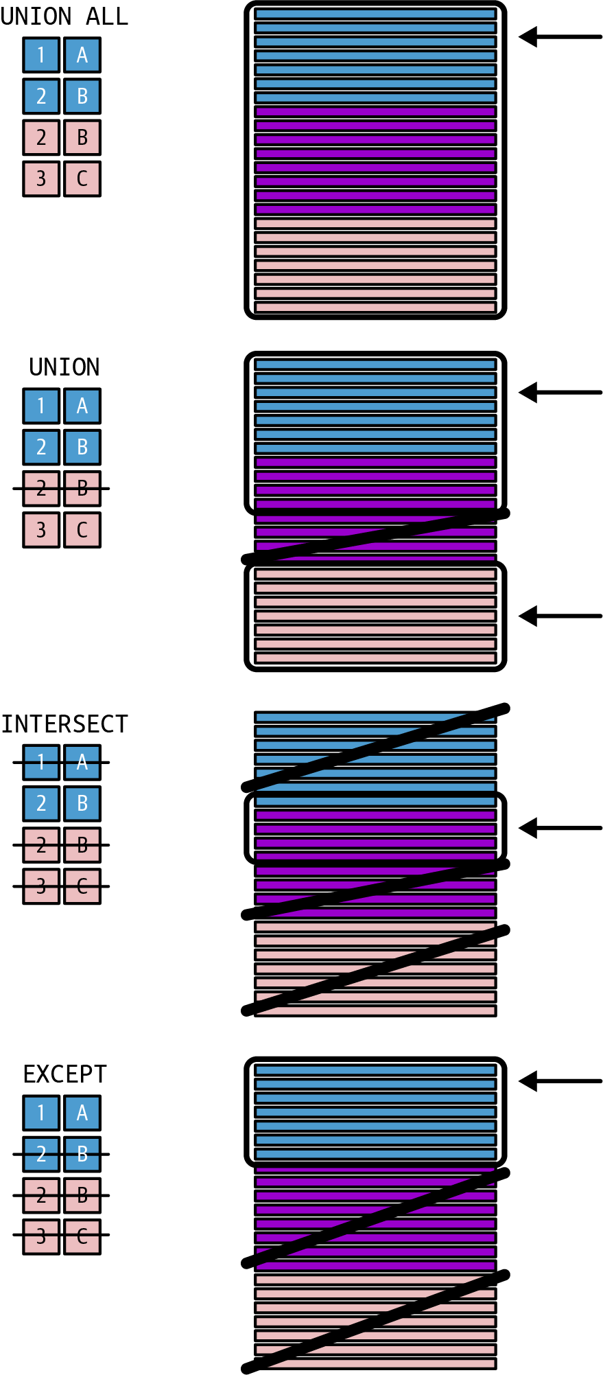
Figure 1-1. Set operators

Warning

To determine whether a row is identical or not, evaluate and compare the content of all columns of the row of the query. Pay attention here: while the primary keys listed in the result set might be identical, the names or description might differ. Rows with identical keys but different descriptions will not be recognized as identical by a set operator.

As you learned, set operators combine tables in a vertical fashion. They basically append the content of one table to the content of another table. The number of columns cannot change with a set operator. If you need to combine tables in a way where you add columns from one table to the columns of another table, you need to work with join operators.

Joins

Joins are like set operators in the sense that they also combine two (or more) queries (or tables). Depending on the type of the join operator, you might end up with the same number of rows as the first table, more, or fewer rows. With joins, you can also add columns to a query (which you can not do with a set operator).

While set operators compare all columns, joins are done on only a selected (sub)set of columns, which you need to specify (in the so-called join predicate). For the join predicate, you’ll usually use an equality comparison between the primary key of one table and the foreign key in the other table (equi-join). For example, you want to show the name of a customer for a certain order (and specify an equality comparison between the order table’s foreign key [Customer Key] and the customer table’s primary key [Customer Key] in the join predicate).

Only in special cases would you compare other (non-key) columns with each other to join two tables. You will see examples of such joins in Chapters 7, 11, 15, and 19, where I demonstrate solutions to advanced problems. There, you’ll also see examples for non-equi-joins. Non-equi-joins use operators like between, greater than or equal to, not equal, etc., to join the rows of two tables.

One example is about grouping values (binning). Binning is about finding the group a certain value falls into by joining the table containing the groups with a condition asking for values that are greater than or equal to the lower range of the bin and lower than the upper range of the bin. While the range of values form the composite primary key of the table containing the groups, the lookup value is not a foreign key: it’s an arbitrary value, possibly not found as a value in the lookup table, as the lookup table only contains a start and end value per bin, but not all the values within the bin.

Natural joins are a special case of equi-joins. In such a join, you don’t specify the columns to compare. The columns to use for the equi-joins are automatically chosen for you: columns with the same name in the two joined tables are used. As you might guess, this only works if you stick to a naming convention (a very good idea in any case) to support these joins. If the primary key and foreign key columns have different names, a natural join will not work properly (e.g., when the primary key in the customer table is the column ID, while, in the order table, the foreign key is named CustomerID). The same is true in the opposite case, when columns in both tables have the same name but no relationship (e.g., both the Product table and the Product Cat⁠egory table have a Name column, which represents the name of the Product and the name of the Product Category, respectively, but they cannot meaningfully used for the equi-join).

Tip

The important difference between set operators and joins is that joins add columns to the first table, while set operators add rows. Joins allow you to add a category column to your products, which can be found in a lookup table. Set operators allow you to combine, e.g., tables containing sales from different data sources into one unified sales table.

I imagine set operators as a combination of tables arranged vertically (one table underneath another) and join operators as a horizontal combination of tables (side-by-side). This metaphor isn’t exact in all regards (set operators INTERSECT and EXCECPT remove rows, and joins also add or remove rows depending on the cardinality of the relationship or the join type) but it is, I think, a good starting point to differentiate them.

Earlier in this chapter, I used Employee as a typical example, where the foreign key ([Manager Key]) references a row in the same table (via primary key [Employee Key]). If you actually join the Employee table with itself, to find, e.g., the manager’s name for an employee, you are implementing a self-join.

You can join two tables in the following ways:

Inner join

Looks for rows that appear in both tables. Only rows appearing in both tables are kept; all other rows are omitted. For example, you want to get a list of customers for whom you can find orders. You can see a graphical representation in Figure 1-2.

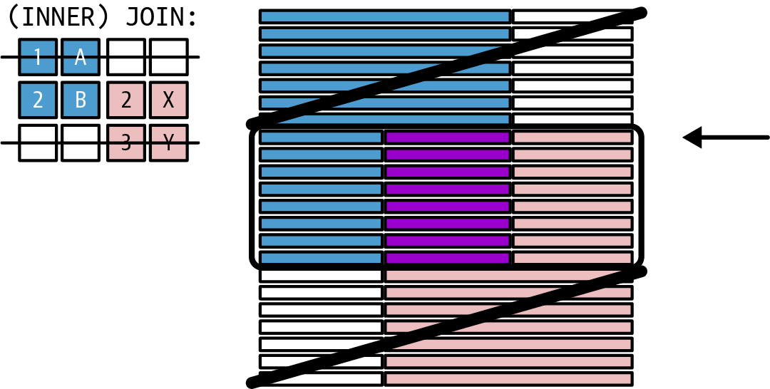
Figure 1-2. Inner join

This is similar to the INTERSECT set operator. But the result can contain the same, more, or fewer rows than the first table. It will contain the same number of rows, if for every row of the first table exactly one row in the second table exists (e.g., when every customer has placed exactly one order). It will contain more rows if there is more than one matching row in the second table (e.g., when every customer has placed at least one order or some customers have so many orders that they overcompensate for customers who didn’t place an order). It will contain fewer rows if some rows of the first table can’t be matched to rows in the second table (e.g., when not all customers have placed orders and these missing orders are not compensated by other customers).

Warning

There is a “danger” of inner joins: the result may skip some rows of one of the tables (e.g., the result will not list customers without orders).

Outer join

Returns all the rows from one table and values for the columns of the other table from matching rows. If no matching row can be found, the value for the columns of the other table are null (and the row of the first table is still kept). This is shown in Figure 1-3.

You can ask for all rows of the first table in a chain of join operators (left join), making the values of the second table optional; the other way around is a right join. A full outer join makes sure to return all rows from both tables (with optional values from the other table).

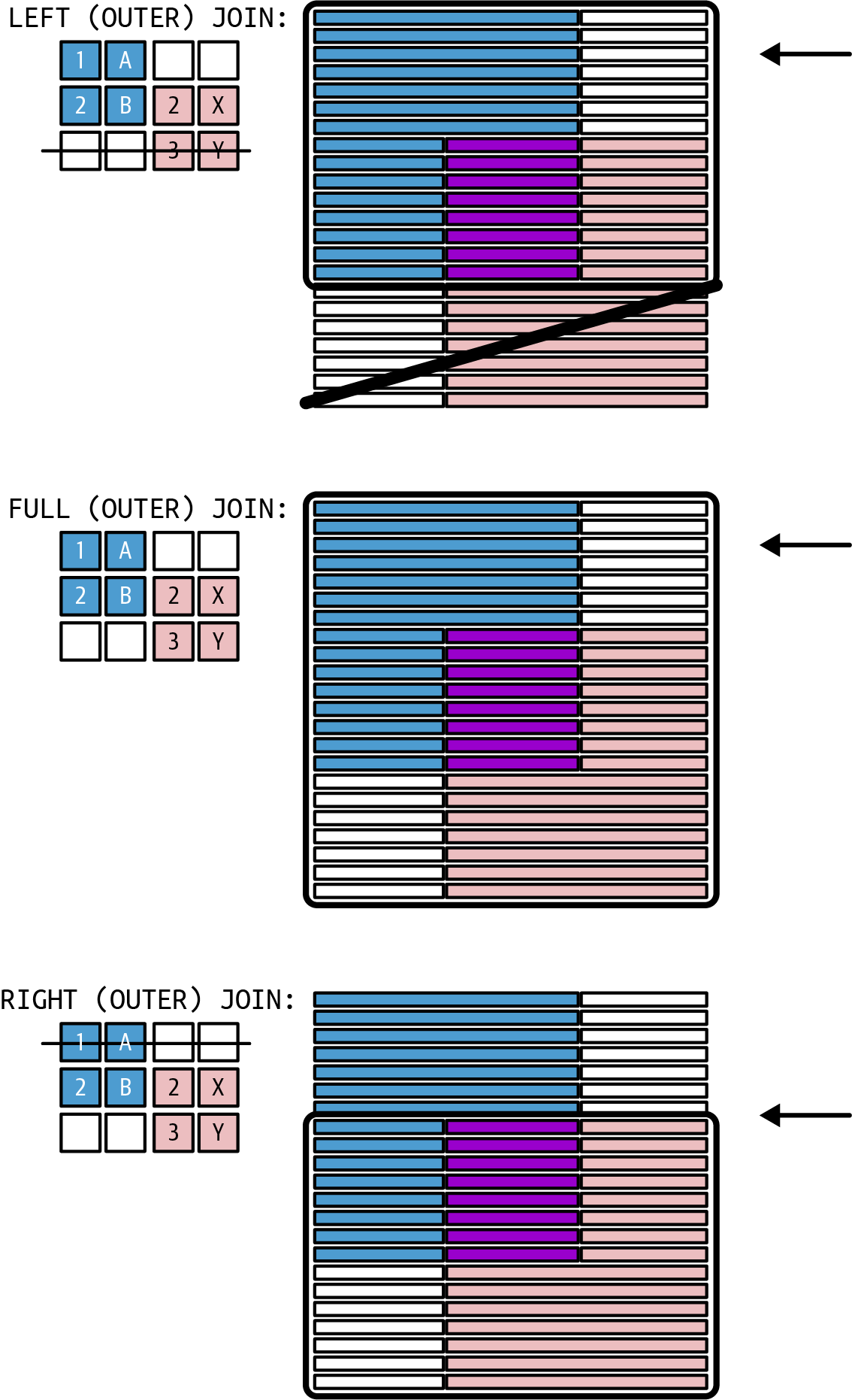
Figure 1-3. Outer join

For example, you want a list of all customers with their order sales from the current year, even when the customer did not order anything in the current year (and then you want null or 0 displayed as their order sales). To achieve this, you would select the rows from the Customer table and left join the Orders table to it. The first table (Customer) is considered the left table, and the joined table (Orders) is the right table in such a query.

Tip

This is easy to understand in SQL when you write all the tables in one single line, e.g., …​FROM Customer LEFT OUTER JOIN Order…​. The Customer table is literally written to the left of the Order table, thus it is the left table. The Order table is literally right of the Customer table, thus it is the right table.

There is no similar set operator to achieve this. An outer join will have at least as many rows as an inner join. It’s not possible that an outer join (with the identical join predicated) will return fewer rows than an inner join. Depending on the cardinality, it might return the same number of rows (if there is a matching row in the second table for every row in the first table) or more (if some rows of the first table cannot be matched with rows of the second table, which are omitted by an inner join).

Anti-join

An anti-join is based on an outer join, where you only keep the rows not existing in the other table. The same ideas apply here for left, right, and full, as you can see in Figure 1-4.

Anti-joins have a very practical use. For example, you want a list of customers who didn’t order anything in the current year (to send them an offer they can’t resist). There is no similar set operator to achieve this. The anti-join delivers the difference between an inner join and an outer join.

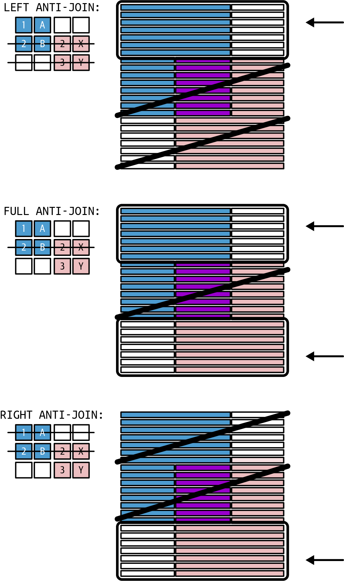
Figure 1-4. Anti-join

Cross join

Creates a so-called Cartesian product. Every single row of the first table is combined with each and every row from the second table. In many scenarios, this doesn’t make sense (e.g., when combining every row of a sales table with every customer without considering whether the row of the sales table is for that customer or a different one).

Practically, you can create queries, which show possible combinations. For example, by applying a cross join on the sizes of clothes with all the colors, you get a list of all conceivable combinations of sizes and colors (independently of if a product really is available in this combination of size and color). A cross join can be a basis for a left join or anti-join, to explicitly point out combinations with no values available. You can see an example of the result of a cross join in Figure 1-5.

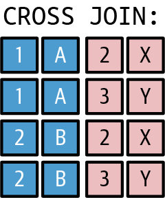
Figure 1-5. Cross join

Do you feel dizzy from all of the join options? Unfortunately, I need to add one more layer of complexity. As you’ve learned, when joining two tables, the number of rows in the result set might be smaller than, equal to, or higher than the number of rows of a single table involved in the operation. The exact number depends on both the type of the join and the cardinality of the tables. In a chain of joins involving several tables, the combined result might lead to undesired results.

Join Path Problems

The Power BI data model has a fail-safe to avoid the join path problems described here. The problems can easily show up, however, when you combine tables in Power Query, in SQL, or your data source.

When you join the rows of one table to the rows of another table, you can face several problems, resulting in unwanted query results: loop, chasm trap, and fan trap. Let’s take a closer look at them.

Loop

You face this problem in a data model if more than one single path exists between two tables. It doesn’t have to be a literal loop in your entity relationship diagram where you can “walk” a join path in a manner where you return to the first table. You’re already talking about a loop when a data model is ambiguous. And this can exist not only in very complex data models but also in the very simple setting of having just more than one direct relationship between the same two tables. Think of a sales table containing a due date, an order date, and a ship date column (Figure 1-6). All three date columns of the table FactResellerSales (DueDateKey, OrderDateKey, and SalesDateKey) have a relationship to the date column of the date table.

The tables contain the following rows (Tables 1-2 and 1-3).

Table 1-2. DimDate

DateKey
2023-08-01
2023-08-02
2023-08-03

Table 1-3. FactResellerSales

DueDateKey	OrderDateKey	ShipDateKey	SalesAmount
2023-08-01	2023-08-01	2023-08-02	10
2023-08-01	2023-08-02	2023-08-02	20
2023-08-01	2023-08-02	2023-08-03	30
2023-08-03	2023-08-03	2023-08-03	40

If you join the DimDate table with the FactResellerSales simultaneously on all three DateKey columns by writing a join predicate like this:

DimDate.DateKey = FactResellerSales.DueDateKey AND DimDate.DateKey =
FactResellerSales.OrderDateKey AND DimDate.DateKey =
FactResellerSales.ShipDateKey

the result would show only a single row (namely the row that—by chance—was due, ordered, and shipped on the same day, 2023-08-03; shown in Table 1-4). We might safely assume that many business orders are not due or shipped on the day of the order. Such sales rows would not be part of the result. This might be an unexpected behavior, returning too few rows.

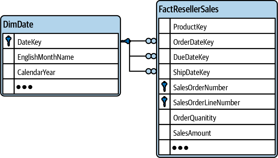
Figure 1-6. Join path problem: loop

Table 1-4. Query result

DateKey	DueDateKey	OrderDateKey	ShipDateKey	SalesAmount
2023-08-03	2023-08-03	2023-08-03	2023-08-03	40

The solution for a loop is (physically or logically) duplicating the date table and joining one date table on the order date and the other date table on the ship date.

Chasm trap

The chasm trap describes a situation in a data model wherein you have a converging many-to-one-to-many relationship (see Figure 1-7). For example, you could store the sales you are making over the internet in a different table than the sales you are making through resellers (see Tables 1-6 and 1-7). Both tables can be filtered over a common table, let’s say a date table (Table 1-5). The date table has a one-to-many relationship to each of the two sales tables—creating a many-to-one-to-many relationship between the two sales tables.

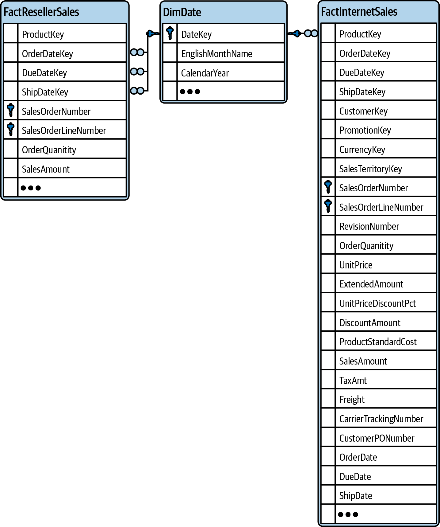
Figure 1-7. Join path problem: chasm trap

Table 1-5. DimDate

DateKey
2023-08-01
2023-08-02
2023-08-03

Table 1-6. FactResellerSales

OrderDateKey	SalesAmount
2023-08-01	10
2023-08-02	20
2023-08-02	30
2023-08-03	40

Table 1-7. FactInternetSales

OrderDateKey	SalesAmount
2023-08-01	100
2023-08-02	200
2023-08-03	300

Joining DimDate and FactResellerSales on DimDate.OrderDateKey = Fact​Resel⁠ler​Sales.OrderDateKey would result in four rows, where the 2023-08-02 row of DateKey will be duplicated (due to the fact that on this day there are two reseller sales). So far so good. The (chasm trap) problem comes when you join the Fac⁠t​Inter⁠net​Sales table to this result (on DimDate.OrderDateKey = Fact​Re⁠seller⁠Sales​.OrderDateKey). As the result of the previous join duplicating the 2023-08-02 row of DimDate, the second join will also duplicate all rows of FactInternetSales for this day. In the example, the row with SalesAmount 200 will appear twice in the result. If you add the numbers up, you will incorrectly report an internet sales amount of 400 for 2023-08-02 in the combined query result. This problem appears independently of using an inner or outer join. (In Table 1-8, I abbreviate FactResellerSales as FRS and FactInternetSales as FIS.)

Table 1-8. Query result

DateKey	FRS.OrderDateKey	FRS.SalesAmount	FIS.OrderDateKey	FIS.SalesAmount
2023-08-01	2023-08-01	10	2023-08-01	100
2023-08-02	2023-08-02	20	2023-08-02	200
2023-08-02	2023-08-02	30	2023-08-02	200
2023-08-03	2023-08-03	40	2023-08-03	300

The solution for the chasm trap problem depends on the tool you are using. Jump to the chapters in the other parts of this book to read how you solve this in Power Query/M and SQL.

Fan trap

You can step into a fan trap in situations where you want to aggregate on a value on the “one” side of a relationship, while joining a table on the “many” side of the same relationship (see Figure 1-8). For example, you could store the freight cost in a sales header table that holds information per order. When you join this table with the sales detail table that holds information per ordered item of the order (which could be multiple per order), you are duplicating the rows from the header table in the query result, therefore duplicating the amount of freight.

Tables 1-9 and 1-10 exemplify this:

Table 1-9. SalesOrderHeader

SalesOrderID	Freight
1	100
2	200
3	300

Table 1-10. SalesOrderDetail

SalesOrderID	SalesOrderLineID	OrderQty
1	1	10
1	2	20
2	1	30
3	1	40

Joining the tables SalesOrderHeader and SalesOrderDetail on the SalesOrderID leads to duplicated rows of the SalesOrderHeader table; the “1” row for Sales​Or⁠der​ID has two order details and will be duplicated. When you naively sum up the Freight, you would falsely report 200, instead of the correct number, 100.

Table 1-11. Query result

SalesOrderID	Freight	SalesOrderLineID	OrderQty
1	100	1	10
1	100	2	20
2	200	1	30
3	300	1	40

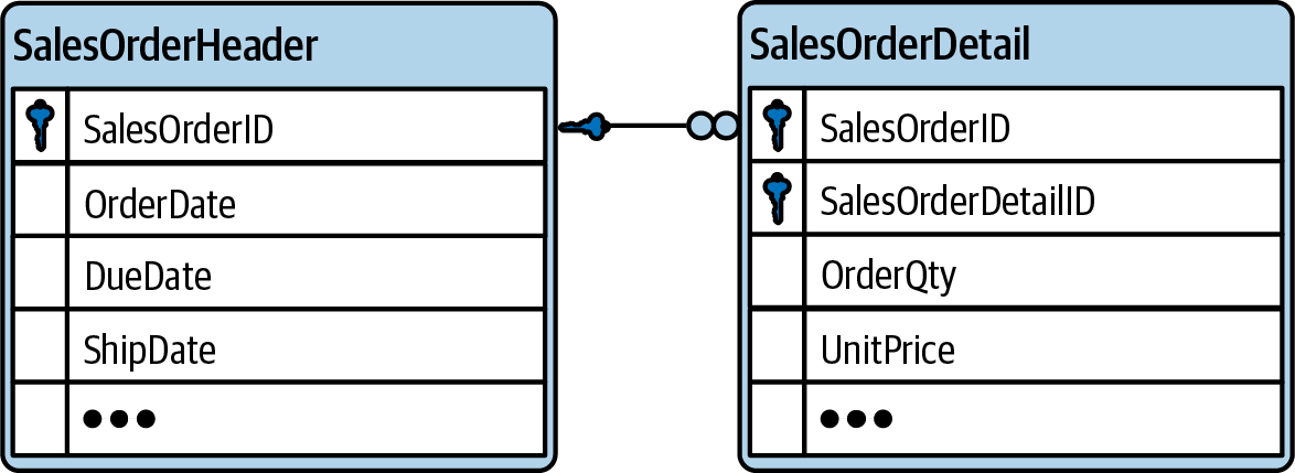
Figure 1-8. Join path problem: fan trap

Similar to the chasm problem, the solution for the fan problem depends on the tool you are using. Jump to the chapters in the other parts of this book to read how you solve this in DAX, Power Query/M and SQL.

As you can see in the screenshots, drawing the tables and the cardinality of their relationships can help in getting an overview about potential problems. The saying “A picture says more than a thousand words” applies to data models as well. I introduce such entity relationship diagrams in the next section.

Entity Relationship Diagrams

An entity relationship diagram (ERD) is a graphical representation of entities and the cardinality of their relationships. When a relationship contains an attribute, it might be shown as a property of the relationship as well. Over the years, different notations have been developed (Lucidchart has a nice overview about the most common notations).

In my opinion, it’s not so important which notation you use—it’s more important to have an ERD on hand for your whole data model. If the data model is very complex (contains a lot of tables) it is common to split it into sections, or sub-ERDs.

Deciding on the cardinality of a relationship and documenting it (e.g., in the form of an ERD) will help you find out in which table you need to create the foreign key. This section explores examples of tables of different cardinality.

The cardinality of the relationship between customers and their orders should be a one-to-many relationship. One customer could have many orders (even when some customers only have a single order or others don’t have any order yet). On the other hand, a particular order is associated with only one customer. This knowledge helps you decide if we need to create a foreign key in the customer table to refer to the primary key of the order table or the other way around. If the customer table contains the [Order Key], it will allow each customer to refer to a single order only, and any order could be referenced by multiple customers. So, plainly, this approach would not correctly reflect the reality. That’s why you need a [Customer Key] (as a foreign key) in the order table instead, as shown in Figure 1-9. Then, every row in the order table can only reference a single customer, and a customer can be referenced by many orders.

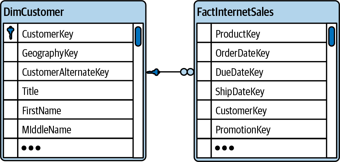
Figure 1-9. ERD for customer and order tables

In a case where an order could be associated with more than a single customer, you would face a many-to-many relationship, as a customer could still have more than one order. Many-to-many relationships are typical if you want to find a data model to represent employees and in which projects they are engaged or collect the reasons for sales from your customers. The same reason will be given for more than one sale, and a customer might give you several reasons for why they made the purchase.

Typically, you would add a foreign key to neither the sales table nor the sales reason table but create a new table on its own consisting of a composite primary key: the primary key of the sales table (SalesOrderNumber and SalesOrderLineNumber in our example, shown in Figure 1-10) and the primary key of the sales reason table (SalesReasonKey). This new table has a many-to-one relationship to the sales table (over the sales table’s primary key) and a many-to-one relationship to the sales reason table (over the sales reason table’s primary key). It’s called a bridge table because it bridges the many-to-many relationship between the two tables and converting it into two one-to-many relationships.

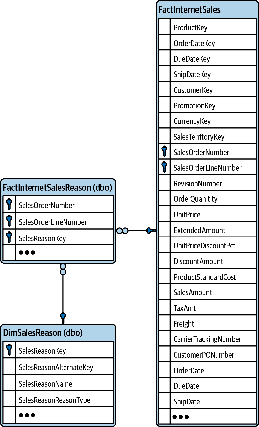
Figure 1-10. ERD for sales and sales reason tables

In later parts of this book, you will learn practical ways to create ERDs for your (existing) data models.

Data Modeling Options

By now, you should have a good understanding of the moving parts of a data model. Therefore, it’s about time we talk about different options for spreading information over tables and relationships in a data model. That’s what the next sections will teach you.

Types of Tables

Basically, you can assign each table in your data model to one of three types:

Entity table

Rows in such a table represent events in the real world. These tables are also referred to as business entity, data, detail, or fact tables. Examples include orders, invoices, etc.

Lookup table

Lookup tables are used to store more detailed information that you don’t want to repeat in every row of the entity table. These tables are also referred to as master, main data, or dimension tables. Examples include customer, product, etc.

Bridge table

A bridge table changes a single many-to-many relationship into two one-to-many relationships. In many database systems, two one-to-many relationships can be handled more gracefully than one many-to-many relationship. For example, you might link a table containing all employees and a table containing all projects.

Maybe you don’t want to split your data into tables but want to keep it in one table. In the next section, I’ll describe the pros and cons of such an idea.

A Single Table to Store It All

Having all necessary information in one single table has its advantages. It’s easily read by humans; therefore, it seems to be a natural way of storing and providing information. If you take a random Excel file, it will probably contain one table (or more) and list all relevant information as columns per a single table. Excel even provides you with functions (e.g., VLOOKUP) to fetch data from a different table to make all necessary information available at one glance. Some tools (e.g., Power BI Report Builder, with which you create paginated reports) require you to collect all information into one query before you can start building a report. If you have a table containing all the necessary information, writing this query is easy, as no joins are involved.

Power BI Desktop and Analysis Services tabular are not those tools. They require you to create a proper data model. A proper data model needs always to consist of more than one table, if you don’t want to encounter difficulties (as “A Single Table to Store It All” points out). In the next section, you will learn rules for splitting columns from one table into several tables to achieve the goal of a redundancy-free data model.

Normal Forms

Codd, the inventor of relational databases, introduced the term normalizing in the context of databases. Personally, I don’t like the term much. I think it’s confusing; it’s hard to tell what’s normal and what’s not, if you think about life in general and databases in particular. But I like the idea and the concept behind this term: the ultimate goal of normalizing a database is to remove redundancy, which is a good idea in many situations.

If you wanted to store the name, address, email, phone, etc. of the customer for each and every order, you could store this information in a redundant manner, requiring you to use more storage space than necessary, due to the duplicated information. Such a solution also makes editing the data overly complicated. You would need to touch not just a single row for the customer but many (in the combined order table) if the content of an attribute changes. If the address of a customer changes, you would need to make sure to change all occurrences of this information over multiple rows. If you want to insert a new customer who just registered in your system but didn’t order anything yet, you have to store a placeholder value in the columns that contain the order information until an order is placed. If you delete an order, you have to pay attention, so as not to accidentally also remove the customer information, in case this was the customer’s only order in the table.

To normalize a database, you apply a set of rules to bring it from one state to the other. Here are the rules to bring a database into the third normal form, which is the most common normal form:¹

Rule of the first normal form (1NF)

You need to define a primary key and remove repeating column values.

Rule of the second normal form (2NF)

Non-key columns are fully dependent on the primary key.

Rule of the third normal form (3NF)

All normal form are directly dependent on the primary key.

Tip

The following sentence has helped me memorize the different rules: each attribute is placed in an entity where it is dependent on the key, the whole key, and nothing but the key…​so help me, Codd (origin unknown).

Let’s apply those rules on a concrete example in Table 1-12.

Table 1-12. A table violating the rules of normalization

StudentNr	Mentor	MentorRoom	Course1	Course2	Course3
1022	Jones	412	101-07	143-01	159-02
4123	Smith	216	201-01	211-02	214-01

This is one single table containing all the necessary information for our hypothetical scenario. In some situations, such a table is very useful, as laid out in “A Single Table to Store It All”. But this is not a good data model, when it comes to Power BI, and it clearly violates all three rules of normalization (you need to define a primary key and remove repeating column values; non-key columns are fully dependent on the primary key; all attributes are directly dependent on the primary key).

In this example, you see repeating columns for the courses a student attends (columns Course1, Course2, and Course3). Such a schema limits the amount of courses to three, and creating a report on how many students visited a certain course is overcomplicated, as you need to look in three different columns. Sometimes information is not split into several columns but all information is stored in a single column, separated by commas, or stored in a JSON or XML format (e.g., a list of phone numbers). Again, querying will be extra hard, as the format of the input cannot be forced. Some might delimet the list using a comma, others might use a semicolon, etc. These examples violate the rule of the first normal form, as well. You need to deserialize the information, and split the information into rows instead, so that you get just one column with the content split out into separate rows. This transforms the table toward 1NF.

Here, somebody might accidentally assign a student to a given course more than once. The database could not prohibit such a mistake. Yes, you could add a check constraint to enforce that the three columns must have different content. But somebody could add a second row for student number 1022, and add course 143-01.

Here, the definition of a primary key comes into play. A primary key uniquely identifies every row of this new table. In this first step, I don’t introduce a new (surrogate) key but can live with a composite primary key. In Table 1-13, the column headers, which make up the primary key, are printed underlined ( StudentNr and Course).

Table 1-13. A table in first normal form (with a composite primary key consisting of StudentNr and Course)

StudentNr	Mentor	MentorRoom	Course
1022	Jones	412	101-07
1022	Jones	412	143-01
1022	Jones	412	159-02
4123	Smith	216	201-01
4123	Smith	216	211-02
4123	Smith	216	214-01

To transform this table into 2NF, start at a table in 1NF and guarantee that all columns are functionally dependent on (all columns of) the primary key. A column is functionally dependent on the primary key if a change in the content of the primary key also requires a change in the content of the column. A look at the table makes it clear that the column Mentor is functionally dependent on the column StudentNr, but apparently not on the column Course. No matter which courses a student attends, his or her mentor stays the same. Mentors are assigned to students in general, not on a by-course basis and the same applies to the column MentorRoom. So you can safely state that columns Mentor and MentorRoom are functionally dependent on only the StudentNr, but not on Course. Therefore, the current design violates the rules for 2NF.

Keeping it like this would allow you to introduce rows with the same student number, but different mentors or mentor rooms, which is not possible from a business logic perspective.

To achieve the 2NF, you have to split the table into two tables. One should contain columns StudentNr, Mentor, and MentorRoom (with StudentNr as its single primary key) (see Table 1-14). A second one should contain StudentNr and Course only (see Table 1-15). Both columns form the primary key of this table.

Table 1-14. Student table in 2NF (with primary key StudentNr)

StudentNr	Mentor	MentorRoom
1022	Jones	412
4123	Smith	216

Table 1-15. StudentCourse table in 2NF (with a composite primary key consisting of StudentNr and Course)

StudentNr	Course
1022	101-07
1022	143-01
1022	159-02
4123	201-01
4123	211-02
4123	214-01

The rules for 3NF require that there is no functional dependency on non-key columns. In our example, the column MentorRoom is functionally dependent on the column Mentor (which is not the primary key) but not on StudentNr (which is the primary key). A mentor keeps using the same room, independent of the mentee. In the current version of the data model, it would be possible to insert rows with wrong combinations of mentor and mentor room.

Therefore, you have to split the data model into three tables (Tables 1-16, 1-17, and 1-18), carving out columns Mentor and MentorRoom into a separate table (with Mentor as the primary key). The second table contains StudentNr (primary key) and Mentor (foreign key to the newly created table). And finally, the third, unchanged table contains StudentNr (foreign key) and Course (which both form the primary key of this table).

Table 1-16. Student table in 3NF (with primary key StudentNr)

StudentNr	Mentor
1022	Jones
4123	Smith

Table 1-17. Mentor table in 2NF (with primary key Mentor)

Mentor	MentorRoom
Jones	412
Smith	216

Table 1-18. The StudentCourse table is in 3NF as well (with a composite primary key consisting of StudentNr and Course)

StudentNr	Course
1022	101-07
1022	143-01
1022	159-02
4123	201-01
4123	211-02
4123	214-01

Table 1-18 is free of any redundancy. Every single piece of information is only stored once. No anomalies or violations to the business logic can happen. This is a perfect data model to store information collected by an application.

The data model is, however, rather complex. This complexity comes with a price: it is hard to understand. It is hard to query (because of many necessary joins). And queries might be slow (because of many necessary joins). These characteristics make this data model less than ideal for analytical purposes. Therefore, I will introduce you to dimensional modeling in the next section.

Dimensional Modeling

Data models in 3NF (fully normalized) avoid any redundancy, which makes them perfect for storing information for applications. Data maintained by applications can rapidly change. Normalization guarantees that a change only has to happen in one place (content of a single column in a single row in on a single table).

Unfortunately, normalized data models are hard to understand. If you look at the ERD of a model for even a simple application, you will be easily overwhelmed by the number of tables and relationships between them. It’s not rare that the printout will cover the whole wall of an office and that application developers who use this data model are only confident about a certain part of the model. If a data model is hard to understand for IT folks, how hard will it then be for domain experts to understand?

Such data models are also hard to query. In the process of normalizing, multiple tables get created, so querying the information in a normalized data model requires you to join multiple tables together. Joining tables is expensive. It requires a lengthy query to be written (and the lengthier, the higher the chance for making mistakes; if you don’t believe me, reread “Joins” and “Join Path Problems”), and it requires you to physically join the information spread out from different tables by the database management system. The more joins, the slower the query.

Therefore, let’s discuss dimensional modeling. You can look at this approach as a (very good) compromise between a single table and a fully normalized data model. Dimensional models are sometimes referred to as denormalized models. As little as I like the term normalized, I dislike the term denormalized even more. Denormalizing can be easily misunderstood as the process to fully reverse all steps done during normalizing. That’s wrong. A dimensional model reintroduces redundancy for some tables, but does not undo all the efforts of bringing a data model into third normal form.

Remember, the ultimate goal is to create a model that’s easy for the report creators to understand and use and allows for fast query performance. A dimensional model is common for data warehouses (DWHs), and Online Analytical Processing (OLAP) systems—also called cubes—and is the optimal model for Power BI and Analysis Services tabular.

In a dimensional model, most of the attributes (or tables) can be either seen as a dimension (hence the name dimensional modeling) or as a fact.²

A dimension table contains answers to How? What? When? Where? Who? Why? The answers are used to filter and group information in a report. This kind of table can and will be wide (it can contain loads of columns). Compared to fact tables, dimension tables will be relatively small in terms of the number of rows (“short”).

Dimension tables are on the “one” side of a relationship. They have a mandatory primary key (so they can be referenced by a fact table) and contain columns of all sorts of data types. In a pure star schema, dimension tables do not contain foreign keys, but are fully denormalized. Think of the number of articles (dimension) a retailer sells, compared to the number of sales transactions (fact).

A fact table tracks real-world events, sometimes called transactions, details, or measurements. It is the core of a data model, and its content is used for counting and aggregating in a report. You should make sure you keep fact tables narrow (add columns only if really necessary), because compared to dimension tables, fact tables can be relatively big in terms of the number of rows (“long”). You want fact tables to be fully normalized.

Fact tables are on the “many” side of a relationship. If there isn’t a special reason, then a fact table won’t contain a primary key because a fact table is not—and never should be—referenced by another table. Every bit you save in each row adds up to a lot of space when multiplied by the number of rows. Typically, you will find foreign keys and (mostly) numeric columns. The latter can be of an additive, semiadditive, or nonadditive nature. Some fact tables contain transactional data, others snapshots or aggregated information.

Depending on how much you denormalize the dimension tables, you will end up with a star schema or a snowflake schema. In a star schema, dimensional tables do not contain foreign keys. All relevant information is already stored in the table in a fully denormalized fashion. That’s what Power BI (and a columnstore index in Microsoft’s relational databases) is optimized for. For certain reasons, you might keep a dimension table (partly) normalized and split information over more than one table. Then, some of the dimension tables will contain a foreign key. A star schema is preferred over a snowflake schema because in comparison, a snowflake schema:

• Has more tables (due to normalization)

• Takes longer to load (because of the bigger amount of tables)

• Makes filtering slower (due to necessary additional joins)

• Makes the model less intuitive (instead of having all information for a single entity in a single table)

• Impedes the creation of hierarchies (in Power BI/Analysis Services tabular)

Of course, a dimension table may contain redundant data, due to denormalizing. In a data warehouse scenario, this isn’t a big issue; there’s only one process that can add and change rows to the dimension table (see “Extract, Transform, Load”).

The number of rows and columns for a fact table will be given by the level of granularity of the information you want or need to store within the data model. It will also give the number of rows of your dimension tables. The next section talks about this important part.

Granularity

Granularity refers to the level of detail of a table. On the one hand, you can define the level of detail of a fact table by the foreign keys it contains. A fact table could track sales per day; or it could track sales per day and product, or by day, product, and customer. This would be three different levels of granularity.

On the other hand, you can also look on the granularity in the following terms:

Transactional fact

The level of granularity is at the event level. All the details of the event are stored (not aggregated values).

Aggregated fact

In an aggregated fact table, some foreign keys might be left out, or you can use a foreign key to a dimension table of different granularity. The fact table might contain sales per day (and reference a “day” dimension table). The aggregated fact table sums up the sales per month (and references a “month” dimension table). Or, you can pick a placeholder value for the existing foreign key (e.g., the first day of the month of the dimension table on the day level) and the rows are grouped and aggregated on the remaining foreign keys. This can make sense when you want to save storage space and/or make queries faster.

An aggregated fact table can be part of a data model additionally related to a transactional fact table, when the storage space is not so important but query performance is. In the chapters about performance tuning, you will learn more about how to improve query time with the help of aggregation tables.

Periodic snapshot fact

When you don’t reduce the number of foreign keys but reduce the granularity of the foreign key on the date table, you have created a periodic snapshot fact table. For example, you keep the foreign key to the date table, but instead of storing events for every day (or multiple events per day), you reference only the (first day of the) month to create a periodic snapshot on the month level. This is common with stock levels and other measures from a balance sheet. Queries are much faster when you have the correct number of available products in stock per day or month, instead of adding up the initial stock and all transactions until the point in time you need to report.

Accumulated snapshot fact

In an accumulated snapshot table, aggregations are done for a whole process. Instead of storing a row for every step of a process (and storing, e.g., the duration of this process), you store only one row, covering all steps of a process (and aggregating all related measures, like the duration).

No matter which kind of granularity you choose, it’s important that a table’s granularity stays constant for all rows of a table. For example, you should not store aggregated sales per day in a table that is already at the granularity level of day and product. Instead, you would create two separate fact tables, one with the granularity of only the day, and a second one with granularity of day and product. It would be complicated to query a table in which some rows are on transactional level, but other rows are aggregated. This would make the life of the report creator hard, and not easy.

Keep also in mind that the granularity of a fact table and the referenced dimension table must match. If you store information by product group in a fact table, it is advised to have a dimension table with the product group as the primary key.

Now that you know how the data model should look, it is time to talk about how you can get the information of your data source into the right shape. The process is called extract, transform, and load, introduced in the next section. In later chapters. I’ll give concrete tips, tricks, and scripts for using Power BI, DAX, Power Query, and SQL to implement transformations.

Extract, Transform, Load

By now, I hope I’ve made clear that a data model that is optimized for an application can look very different from a data model for the same data that is optimized for analytics. The process of converting the data model from one type to another is called extract, transform, and load (ETL):

Extract

Extract means to get the data out of the data source. Sometimes the data source offers an API, sometimes it is extracted as files, and sometimes you can query tables in the application’s database.

Transform

Transforming the source data starts with easy tasks such as giving tables and columns user-friendly names (nobody wants to see, say, column EK4711 in a report), and covers data cleaning, filtering, enriching, etc. This is where converting the shapes of the tables into a dimensional model happens. In the “Building a Data Model” sections of each part, you’ll learn concepts and techniques to achieve this.

Load

Because the source system might not be available 24/7 for analytical queries (or ready for such queries at all) and transformation can be complex as well, storing extracted and transformed data so that it can be queried quickly and easily is recommended (e.g., in a Power BI semantic model in the Power BI service or in an Analysis Services database). Storing it in a relational data warehouse (before making it available to Power BI or Analysis Services) makes sense in most enterprise environments.

The ETL process is sometimes compared to tasks in a restaurant kitchen. The cooks have dedicated tools to process the food and use all their knowledge and skills to make the food both good-looking and tasty, when served on a plate to the restaurant’s customer. It’s a great analogy for what happens during ETL because we use tools, knowledge, and skills to transform raw data into savory data that encourages an appetite for insights (hence the name of my company). Such data can then easily be consumed to create reports and dashboards.

Because the challenge of extracting, transforming, and loading data from one system to another is widespread, plenty of tools are available. Common tools in Microsoft’s Data Platform family are SQL Server Integration Services, Azure Data Factory, Power Query, and Power BI dataflows. You should have one single ETL job (e.g., one SQL Server Integration Services package, one Azure Data Factory pipeline, one Power Query query or one Power BI dataflow) per entity in your data warehouse. Then it’s straightforward to adopt the job in case the table changes. These jobs are then put into the correct order by one additional orchestration job.

Sometimes people refer not to ETL, but to ELT or ELTLT, as the data might be first loaded into a staging area and then transformed. I personally don’t think it so important if you first load the data and then transform it, or the other way around. The order is mostly determined by which tool you are using (if you need or ought to first persist data before you transform it, or if you can transform it “on-the-fly” when loading the data). The most important thing is that the final result of the whole process must be accessible easily and quickly by the report users, to make their life easier (as postulated in the introduction to this chapter).

Implementing all transformations before users query the data is crucial, as is applying transformations as early as possible. If you possess a data warehouse, then implement the transformations there (via SQL Server Integration Services, Azure Data Factory, or simply views). If you don’t have (access to) a data warehouse, then implement and share the transformations as Power BI dataflow or use Power Query (inside Power BI Desktop) and share the result as a Power BI semantic model.

Only implement the transformations in the report layer as a last resort (better to implement it there instead of not implementing it at all). The “earlier” in your architecture you implement the transformation, the more tools can be employed, and the more accessible your product will be for users (like data engineers, data scientists, analysts, etc.). Something implemented only in the report is only available to the users of the report. If you need the same logic in another report, you need to re-create the transformation there (and face all consequences of code duplication, like a higher maintenance effort for code changes and the risk of different implementations of the same transformation, leading to different results).

If you do the transformation in Power Query (in Power BI or in Analysis Services), then only users and tools with access to the Power BI semantic model or Analysis Services tabular database benefit from them. When you implement everything in the data warehouse layer (which might be a relational database, but could be a data lake or delta lake as well, or anything else that can hold all the necessary data and allows for your transformations), then a more widespread population of your organization will have access to clean and transformed information, without transformations needing to be repeated. You can connect Power BI to those tables and not need to apply any transformations.

Every concept introduced so far is based on the great work of two giants of data warehousing: Ralph Kimball and Bill Inmon.

Ralph Kimball and Bill Inmon

A book about data modeling would not be complete without mentioning (and referencing) Ralph Kimball and Bill Inmon. Both are the godfathers of data warehousing. They invented many concepts and solutions for different problems you will face when creating an analytical database. Their approaches have some things in common but show also huge differences. Regarding their differences, they never found compromises, and they “fought” about them (and against each other) in their articles and books.

For both, dimensional modeling (facts and dimensions) play an important role as the access layer for the users and tools. Both call this layer a data mart. But they describe the workflow and the architecture to achieve this quite differently.

For Kimball, the data mart comes first. A data mart contains only what is needed for a certain problem, project, workflow, etc. A data warehouse does not exist on its own but is just the collection of all available data marts in your organization. The data marts are shaped in a star schema fashion. Even when “Agile project management” wasn’t (yet) a thing, when Kimball described his concept, they clearly matched easily. Concentrating on smaller problems and creating data marts for them allows for quick wins. Of course, there is a risk that you won’t always keep the big picture in mind and end up with a less consistent data warehouse, as dimensions are not as conformed as they should be over the different data marts.

Kimball invented the concept of an Enterprise Data Bus to make all dimensions conform. He retired in 2015, but you can find useful information at The Kimball Group, and his books are still worth a read. Their references and examples to SQL are still valid. He didn’t mention Power BI or the Analysis Services tabular model, which were only emerging then.

On the other hand, Inmon favors a top-down approach: you need to create a consistent data warehouse in first place. He called this central database the Corporate Information Factory, and it is fully normalized. Data marts are then derived from the Corporate Information Factory where needed (by denormalizing the dimensions into a star schema). While this will guarantee a consistent database and data model, it surely will lead to a longer project duration while you collect all requirements and implement them in a then consistent fashion. His ideas are collected in Building the Data Warehouse, 4th Ed. (Wiley, 2005) and are worth read as well. Inmon also supports the Data Vault modeling approach (“Data Vaults and Other Anti-Patterns”) and is an active publisher of books around data lake architecture.

If you want to dig deeper into the concept of a star schema (which you should!) I strongly recommend reading Chris Adamson’s masterpiece Star Schema: The Complete Reference (McGraw Hill, 2010).

Over the years, many different data modeling concepts have been developed and many different tools to build reports and support ad hoc analysis have been created. In the next section, I describe them as anti-patterns. Not because they are bad in general, but because Power BI and Analysis Services tabular are optimized for the star schema instead.

Data Vaults and Other Anti-Patterns

I won’t go into many details of how you can implement a Data Vault architecture. It is, however, important to lay out that a Data Vault is merely a data modeling approach that makes your ETL process flexible and robust against changes in the structure of the data source. The Data Vault’s philosophy is to postpone cleaning of data to when it reaches the business layer. As easy as this approach makes the lives of data warehouse/ETL developers is proportional to how difficult it will make the lives of the business users. Remember: this book aims to describe how you can create a data model that makes the end user’s life easier.

A Data Vault model is somewhere between a 3NF and a star schema. Proponents of the Data Vault claim rightfully that such a data model can also be loaded into Power BI or Analysis Service Tabular. There is a problem, though: you can load any data model into Power BI and Analysis Services tabular—but you will pay a price when it comes to query performance (this happened to me with the first data model I implemented with Power BI; even when the tables contained just a few hundred rows, the reports I built were really slow). You will sooner or later suffer from overcomplicated DAX calculations too.

That’s why I strongly recommend that you not use any of the following data model approaches for Power BI and Analysis Services tabular:

Single table

See my reasoning in “A Single Table to Store It All”.

A table for every source file

This is a trap non-IT users easily step into. A table should contain attributes of only one entity. Often, a flat file or an Excel spreadsheet contains a report and not information limited to one entity. Chances are high that when you create a data model with one table per file, the same information is spread out over different tables, and that many of your relationships will show a many-to-many cardinality due to a lack of primary keys. Applying filters on those attributes and writing more than just simple calculations can quickly start to be a nightmare. Sometimes this “model” is referred to as OBT (one big table).

Fully normalized schema

Such a schema is optimized for writing, not for querying. The number of tables and necessary joins makes it hard to use and impairs query response times. Chances are high that query performance is less than optimal, and that you will suffer from join path problems (see “Join Path Problems”).

Header—detail

Separating things like the order information and the order line information into two tables requires you to join two relatively big tables (as you will have loads of orders and loads of order lines, representing the different goods, per order). This additional join will make queries slow and DAX more complex than necessary, compared to combining the header and detail table into just one fact table. The joined table will contain as many rows as the detail table already has and as many columns as the two tables combined, except for the join key column, but will save the database management system from executing joins over two big tables.

Key-value

A key-value table is a table with basically just two columns: a key column (containing, e.g., the string Sales) and a value column (containing, e.g., 100). Such a table is very flexible to maintain (for new information, you just add a new row with a new key, e.g., “Quantity”), but it is very hard to query. In Chapter 3, I write at length about the challenges key-value-pair tables bring, and how to overcome them in order to transform them into a meaningful table.

The reason I describe these as anti-patterns is not that these modeling approaches, from an objective point of view, are worse than star schema. The only reason is that many reporting tools benefit from a star schema so much that it is worthwhile to transform your data model into one. The only exceptions are tools like Power BI paginated reports, which benefit from (physical or virtual) single tables containing all the necessary information.

The VertiPaq engine (which is the storage engine behind Power BI, Analysis Services tabular, Excel’s Power Pivot and SQL Server’s columnstore index) is fully optimized for star schemas with every single fiber. You should not ignore this fact.

While you can write a letter in Excel and do some simple calculations in a table in a Word document, there are good reasons why you would write a letter with Word and create the table and its calculations in Excel. You would not start complaining about how hard it is to write a letter in Excel or that many features to do your table calculations are missing in Word. Your mindset toward Power BI should be similar: you can use any data model in Power BI, but you should not start complaining about the product unless you have your data modeled as star schema.

Key Takeaways

Congratulations on finishing the first chapter of this book. I am convinced that all the described concepts are crucial for your understanding of data models in general, and for all the transformations and advanced concepts coming up in the rest of the book. Here is a short refresher of what you’ve learned so far:

• The basic parts of a data model: tables, columns, relationships, primary keys, and foreign keys.

• Different ways of combining tables with the help of set operators and joins, and which kind of problems you can face when joining tables.

• Normalized data models are optimized for write operations, and that’s why they are the preferred data model for application databases. Dimensional modeling re-introduces some redundancy to make them easier to understand and to allow for faster queries (because fewer joins are necessary).

• Transforming of the data model (and much more) during the ETL process, which extracts, transforms, and loads data from data sources into the data warehouse.

• A rough overview about the contrary ideas of the two godfathers of data warehouses, Ralph Kimball and Bill Inmon.

• Why it is so important to stick to a star schema when it comes to Power BI and Analysis Services tabular.

¹ If you want to dig deeper, you will find books explaining the Boyce–Codd, fourth and fifth normal forms, which I consider mainly of academic interest, and less practically relevant.

² Later I’ll introduce you to other types of tables as well.