Chapter 1. Introduction to Apache Iceberg
Data is a primary asset from which organizations curate the information and insights needed to make critical business decisions. Whether it is used to analyze trends in annual sales of a particular product or to predict future market opportunities, data shapes the direction for organizations to follow to be successful. Further, today data isn’t just a nice-to-have. It is a requirement, not just for winning in the market but for competing in it. With such a massive demand for information, there has been an enormous effort to accumulate the data generated by the various systems within an organization to derive insights.
At the same time, the rate at which operational and analytical systems have been generating data has skyrocketed. While more data has presented enterprises the opportunity to make better-informed decisions, there is also a dire need to have a platform that stores and analyzes all this data so that it can be used to build analytical products such as business intelligence (BI) reports and machine learning (ML) models to support decision making. Lakehouse architecture, which we will elaborate on in this chapter, decouples how we store our data from how we process it for more flexibility. This chapter will walk you through the history and evolution of data platforms from a practical point of view and present the benefits of a lakehouse architecture with Apache Iceberg open table formats.
How Did We Get Here? A Brief History
In terms of storage and processing systems, relational database management systems (RDBMSs) have long been a standard option for organizations to keep a record of all their transactional data. For example, say you run a transportation company and you wanted to maintain information about new bookings made by your customers. In this case, each new booking would be a new row in an RDBMS. RDBMSs used for this purpose support a specific data processing category called online transaction processing (OLTP). Examples of OLTP-optimized RDBMSs are PostgreSQL, MySQL, and Microsoft SQL Server. These systems are designed and optimized to enable you to interact very quickly with one or a few rows of data at a time and are a good choice for supporting a business’s day-to-day operations.
But say you wanted to understand the average profit you made on all your new bookings from the preceding quarter. In that case, using the data stored in an OLTP-optimized RDBMS would have led to significant performance problems once your data got large enough. Some of the reasons for this include the following:
Transactional systems are focused on inserting, updating, and reading a small subset of rows in a table, so storing the data in a row-based format is ideal. However, analytics systems usually focus on aggregating certain columns or working with all the rows in a table, making a columnar structure more advantageous.
Running transactional and analytics workloads on the same infrastructure can result in a competition for resources.
Transactional workloads benefit from normalizing the data into several related tables that are joined if needed, while analytics workloads may perform better when the data is denormalized into the same table to avoid large-scale join operations.
Now imagine that your organization had a large number of operational systems that generated a vast amount of data and your analytics team wanted to build dashboards that relied on aggregations of the data from these different data sources (i.e., application databases). Unfortunately, OLTP systems are not designed to deal with complex aggregate queries involving a large number of historical records. These workloads are known as online analytical processing (OLAP) workloads. To address this limitation, you would need a different kind of system optimized for OLAP workloads. It was this need that prompted the development of the lakehouse architecture.
Foundational Components of a System Designed for OLAP Workloads
A system designed for OLAP workloads is composed of a set of technological components that enable supporting modern-day analytical workloads, as showcased in Figure 1-1 and described in the following subsections.
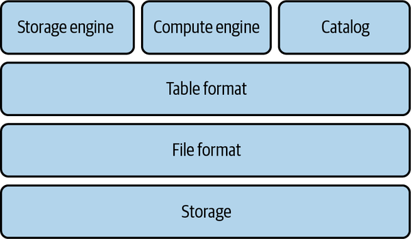
Figure 1-1. Technical components supporting analytical workloads
Storage
To analyze historical data coming in from a variety of sources, you need to have a system that allows you to store large to significant amounts of data. Therefore, storage is the first component you would need in a system that can deal with analytical queries on large datasets. There are many options for storage, including a local filesystem on direct-attached storage (DAS); a distributed filesystem on a set of nodes that you operate, such as the Hadoop Distributed File System (HDFS); and object storage provided as a service by cloud providers, such as Amazon Simple Storage Service (Amazon S3).
Regarding the types of storage, you could use row-oriented databases or columnar databases, or you could mix the two in some systems. In recent years, columnar databases have enjoyed tremendous adoption as they have proven to be more efficient when dealing with vast volumes of data.
File format
For storage purposes, your raw data needs to be organized in a particular file format. Your choice of file format impacts things such as the compression of the files, the data structure, and the performance of a given workload.
File formats generally fall into three high-level categories: structured (CSV), semistructured (JSON), and unstructured (text files). In the structured and semistructured categories, file formats can be row oriented or column oriented (columnar). Row-oriented file formats store all the columns of a given row together, while column-oriented file formats store all the rows of a given column together. Two common examples of row-oriented file formats are comma-separated values (CSV) and Apache Avro. Examples of columnar file formats are Apache Parquet and Apache ORC.
Depending on the use case, certain file formats can be more advantageous than others. For example, row-oriented file formats are generally better if you are dealing with a small number of records at a time. In comparison, columnar file formats are generally better if you are dealing with a sizable number of records at a time.
Table format
The table format is another critical component for a system that can support analytical workloads with aggregated queries on a vast volume of data. The table format acts like a metadata layer on top of the file format and is responsible for specifying how the datafiles should be laid out in storage.
Ultimately, the goal of a table format is to abstract the complexity of the physical data structure and facilitate capabilities such as Data Manipulation Language (DML) operations (e.g., doing inserts, updates, and deletes) and changing a table’s schema. Modern table formats also bring in the atomicity and consistency guarantees required for the safe execution of DML operations on the data.
Storage engine
The storage engine is the system responsible for actually doing the work of laying out the data in the form specified by the table format and keeping all the files and data structures up-to-date with the new data. Storage engines handle some of the critical tasks, such as physical optimization of the data, index maintenance, and getting rid of old data.
Catalog
When dealing with data from various sources and on a larger scale, it is important to quickly identify the data you might need for your analysis. A catalog’s role is to tackle this problem by leveraging metadata to identify datasets. The catalog is the central location where compute engines and users can go to find out about the existence of a table, as well as additional information such as the table name, table schema, and where the table data is stored on the storage system. Some catalogs are internal to a system and can only be directly interacted with via that system’s engine; examples of these catalogs include Postgres and Snowflake. Other catalogs, such as Hive and Project Nessie, are open for any system to use. Keep in mind that these metadata catalogs aren’t the same as catalogs for human data discovery, such as Colibra, Atlan, and the Dremio Software internal catalog.
Compute engine
The compute engine is the final component needed to efficiently deal with a massive amount of data persisted in a storage system. A compute engine’s role in such a system would be to run user workloads to process the data. Depending on the volume of data, computation load, and type of workload, you can utilize one or more compute engines for this task. When dealing with a large dataset and/or heavy computational requirements, you might need to use a distributed compute engine in a processing paradigm called massively parallel processing (MPP). A few examples of MPP-based compute engines are Apache Spark, Snowflake, and Dremio.
Bringing It All Together
Traditionally for OLAP workloads, these technical components have all been tightly coupled into a single system known as a data warehouse. Data warehouses allow organizations to store data coming in from a variety of sources and run analytical workloads on top of the data. In the next section, we will discuss in detail the capabilities of a data warehouse, how the technical components are integrated, and the pros and cons of using such a system.
The Data Warehouse
A data warehouse or OLAP database is a centralized repository that supports storing large volumes of data ingested from various sources such as operational systems, application databases, and logs. Figure 1-2 presents an architectural overview of the technical components of a data warehouse.
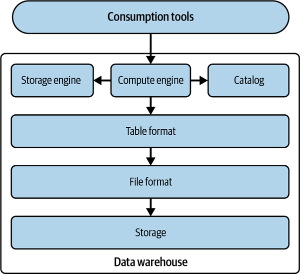
Figure 1-2. Technical components of a data warehouse
A data warehouse owns all the technical components in a single system. In other words, all the data is stored in its proprietary file and table formats on its proprietary storage system. This data is then managed exclusively by the data warehouse’s storage engine, is registered in its catalog, and can be accessed only by the user or analytical engines through its compute engine.
A Brief History
Up until about 2015, most data warehouses had the storage and compute components tightly coupled on the same nodes, since most were designed and run on premises. However, this resulted in a lot of problems. Scaling became a big issue because datasets grew in volume at an accelerating pace while the number and intensity of workloads (i.e., compute tasks running on the warehouse) also increased. Specifically, there was no way to independently increase the compute and storage resources depending on your tasks. If your storage needs grew more quickly than your compute needs, it didn’t matter. You still had to pay for additional compute even though you didn’t need it.
This led to the next generation of data warehouses being built with a big focus on the cloud. These data warehouses began gaining traction around 2015 as cloud-native computing burst onto the scene, allowing you to separate the compute and storage components and scale these resources to suit your tasks. They even allowed you to shut down compute when you weren’t using it and not lose your storage.
Pros and Cons of a Data Warehouse
While data warehouses, whether on premises or cloud based, make it easy for enterprises to quickly make sense of all their historical data, there are certain areas where a warehouse still causes issues. Table 1-1 lists the pros and cons of a data warehouse.
| Pros | Cons |
|---|---|
| Serves as the single source of truth as it allows storing and querying data from various sources | Locks the data into a vendor-specific system that only the warehouse’s compute engine can use |
| Supports querying vast amounts of historical data, enabling analytical workloads to run quickly | Expensive in terms of both storage and computation; as the workload increases, the cost becomes hard to manage |
| Provides effective data governance policies to ensure that data is available, usable, and aligned with security policies | Mainly supports structured data |
| Organizes the data layout for you, ensuring that it’s optimized for querying | Does not enable organizations to natively run advanced analytical workloads such as ML |
| Ensures that data written to a table conforms to the technical schema |
A data warehouse acts as a centralized repository for organizations to store all their data coming in from a multitude of sources, allowing data consumers such as analysts and BI engineers to access data easily and quickly from one single source to start their analysis. In addition, the technological components powering a data warehouse enable you to access vast volumes of data while supporting BI workloads to run on top of it.
Although data warehouses have been elemental in the democratization of data and allowed businesses to derive historical insights from varied data sources, they are primarily limited to relational workloads. For example, returning to the transportation company example from earlier, say that you wanted to derive insights into how much you will make in total sales in the next quarter. In this case, you would need to build a forecasting model using historical data. However, you cannot achieve this capability natively with a data warehouse as the compute engine, and the other technical components are not designed for ML-based tasks. So your main viable option would be to move or export the data from the warehouse to other platforms supporting ML workloads. This means you would have data in multiple copies, and having to create pipelines for each data movement can lead to critical issues such as data drift and model decay when pipelines move data incorrectly or inconsistently.
Another hindrance to running advanced analytical workloads on top of a data warehouse is that a data warehouse only supports structured data. But the rapid generation and availability of other types of data, such as semistructured and unstructured data (JSON, images, text, etc.), has allowed ML models to reveal interesting insights. For our example, this could be understanding the sentiments of all the new booking reviews made in the preceding quarter. This ultimately would impact an organization’s ability to make future-oriented decisions.
There are also specific design challenges in a data warehouse. Returning to Figure 1-2, you can see that all six technical components are tightly coupled in a data warehouse. Before you understand what that implies, an essential thing to observe is that both file and table formats are internal to a particular data warehouse. This design pattern leads to a closed form of data architecture. It means that the actual data is accessible only using the data warehouse’s compute engine, which is specifically designed to interact with the warehouse’s table and file formats. This type of architecture leaves organizations with a massive concern about locked-in data. With the increase in workloads and the vast volumes of data ingested to a warehouse over time, you are bound to that particular platform. And that means your analytical workloads, such as BI and any future tools you plan to onboard, can only run on top of this particular data warehouse. This also prevents you from migrating to another data platform that can cater specifically to your requirements.
Additionally, a significant cost factor is associated with storing data in a data warehouse and using the compute engines to process the data. This cost only increases with time as you increase the number of workloads in your environment, thereby invoking more compute resources. In addition to the monetary costs, there are other overheads, such as the need for engineering teams to build and manage numerous pipelines to move data from operational systems, and delayed time-to-insight on the part of data consumers. These challenges have prompted organizations to seek alternative data platforms that allow data to be within their control and stored in open file formats, thereby allowing downstream applications such as BI and ML to run in parallel with much-reduced costs. This led to the emergence of data lakes.
The Data Lake
While data warehouses provided a mechanism for running analytics on structured data, they still had several issues:
A data warehouse could only store structured data.
Storage in a data warehouse is generally more expensive than on-prem Hadoop clusters or cloud object storage.
Storage and compute in traditional on-prem data warehouses are often commingled and therefore cannot be scaled separately. More storage costs came with more compute costs whether you needed the compute power or not.
Addressing these issues required an alternative storage solution that was cheaper and could store all your data without the need to conform to a fixed schema. This alternative solution was the data lake.
A Brief History
Originally, you’d use Hadoop, an open source, distributed computing framework, and its HDFS filesystem component to store and process large amounts of structured and unstructured datasets across clusters of inexpensive computers. But it wasn’t enough to just be able to store all this data. You’d want to run analytics on it too.
The Hadoop ecosystem included MapReduce, an analytics framework from which you’d write analytics jobs in Java and run them on the Hadoop cluster. Writing MapReduce jobs was verbose and complex, and many analysts are more comfortable writing SQL than Java, so Hive was created to convert SQL statements into MapReduce jobs.
To write SQL, a mechanism to distinguish which files in your storage are part of a particular dataset or table was needed. This resulted in the birth of the Hive table format, which recognized a directory and the files inside it as a table.
Over time, people moved away from using Hadoop clusters to using cloud object storage (e.g., Amazon S3, Minio, Azure Blob Storage), as it was easier to manage and cheaper to use. MapReduce also fell out of use in favor of other distributed query engines such as Apache Spark, Presto, and Dremio. What did stick around was the Hive table format, which became the standard in the space for recognizing files in your storage as singular tables on which you can run analytics. However, cloud storage required more network costs in accessing those files, which the Hive format architecture didn’t anticipate and which led to excessive network calls due to Hive’s dependence on the table’s folder structure.
A feature that distinguishes a data lake from a data warehouse is the ability to leverage different compute engines for different workloads. This is important because there has never been a silver-bullet compute engine that is best for every workload and that can scale compute independently of storage. This is just inherent to the nature of computing, since there are always trade-offs, and what you decide to trade off determines what a given system is good for and what it is not as well suited for.
Note that in data lakes, there isn’t really any service that fulfills the needs of the storage engine function. Generally, the compute engine decides how to write the data, and then the data is usually never revisited and optimized, unless entire tables or partitions are rewritten, which is usually done on an ad hoc basis. Figure 1-3 depicts how the components of a data lake interact with one another.
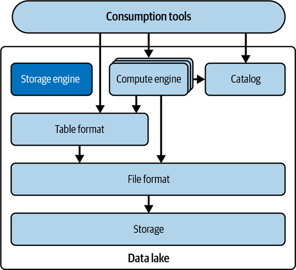
Figure 1-3. Technical components of a data lake
Pros and Cons of a Data Lake
Of course, no architectural pattern is perfect, and that applies to data lakes. While data lakes have a lot of benefits, they also have several limitations. The following are the benefits:
- Lower cost
The costs of storing data and executing queries on a data lake are much lower than in a data warehouse. This makes a data lake particularly useful for enabling analytics on data whose priority isn’t high enough to justify the cost of a data warehouse, enabling a wider analytical reach.
- Stores data in open formats
In a data lake, you can store the data in any file format you like, whereas in a data warehouse, you have no say in how the data is stored, which would typically be a proprietary format built for that particular data warehouse. This allows you to have more control over the data and consume the data in a greater variety of tools that can support these open formats.
- Handles unstructured data
Data warehouses can’t handle unstructured data such as sensor data, email attachments, and logfiles, so if you wanted to run analytics on unstructured data, the data lake was the only option.
These are the limitations:
- Performance
Since each component of a data lake is decoupled, many of the optimizations that can exist in tightly coupled systems are absent, such as indexes and ACID (Atomicity, Consistency, Isolation, Durability) guarantees. While they can be re-created, it requires a lot of effort and engineering to cobble the components (storage, file format, table format, engines) in a way that results in performance comparable to that of a data warehouse. This made data lakes undesirable for high-priority data analytics where performance and time mattered.
- Requires lots of configuration
As previously mentioned, creating a tighter coupling of your chosen components with the level of optimizations you’d expect from a data warehouse would require significant engineering. This would result in a need for lots of data engineers to configure all these tools, which can also be costly.
- Lack of ACID transactions
One notable drawback of data lakes is the absence of built-in ACID transaction guarantees that are common in traditional relational databases. In data lakes, data is often ingested in a schema-on-read fashion, meaning that schema validation and consistency checks occur during data processing rather than at the time of ingestion. This can pose challenges for applications that require strong transactional integrity, such as financial systems or applications dealing with sensitive data. Achieving similar transactional guarantees in a data lake typically involves implementing complex data processing pipelines and coordination mechanisms, adding to the engineering effort required for critical use cases. While data lakes excel at scalability and flexibility, they may not be the ideal choice when strict ACID compliance is a primary requirement.
Table 1-2 summarizes these pros and cons.
| Pros | Cons |
|---|---|
| Lower cost Stores data in open formats Handles unstructured data Supports ML use cases |
Performance Lack of ACID guarantees Lots of configuration required |
Should I Run Analytics on a Data Lake or a Data Warehouse?
While data lakes provided a great place to land all your structured and unstructured data, there were still imperfections. After running ETL (extract, transform, and load) to land your data in your data lake, you’d generally take one of two tracks when running analytics.
For instance, you could set up an additional ETL pipeline to create a copy of a curated subset of data that is for high-priority analytics and store it in the warehouse to get the performance and flexibility of the data warehouse.
However, this results in a few issues:
Additional costs in the compute for the additional ETL work and in the cost to store a copy of data you are already storing in a data warehouse where the storage costs are often greater
Additional copies of the data, which may be needed to populate data marts for different business lines and even more copies as analysts create physical copies of data subsets in the form of BI extracts to speed up dashboards, leading to a web of data copies that are hard to govern, track, and keep in sync
Alternatively, you could use query engines that support data lake workloads, such as Dremio, Presto, Apache Spark, Trino, and Apache Impala, to execute queries on the data lake. These engines are generally well suited for read-only workloads. However, due to the limitations of the Hive table format, they run into complexity when trying to update the data safely from the data lake.
As you can see, data lakes and data warehouses have their own unique benefits and limitations. This necessitated the need to develop a new architecture that offers their benefits while minimizing their faults, and that architecture is called a data lakehouse.
The Data Lakehouse
While using a data warehouse gave us performance and ease of use, analytics on data lakes gave us lower costs, flexibility by using open formats, the ability to use unstructured data, and more. The desire to thread the needle leads to great strides and innovation, which leads to what we now know as the data lakehouse.
The data lakehouse architecture decouples the storage and compute from data lakes and brings in mechanisms that allow for more data warehouse–like functionality (ACID transactions, better performance, consistency, etc.). Enabling this functionality are data lake table formats that eliminate all the previous issues with the Hive table format. You store the data in the same places you would store it with a data lake, you use the query engines you would use with a data lake, and your data is stored in the same formats it would be stored in on a data lake. What truly transforms your world from “read-only” data to a “center of my data world” data lakehouse is the table format providing a metadata/abstraction layer between the engine and storage for them to interact more intelligently (see Figure 1-4).
Table formats create an abstraction layer on top of file storage that enables better consistency, performance, and ACID guarantees when working with data directly on data lake storage, leading to several value propositions:
- Fewer copies = less drift
With ACID guarantees and better performance you can now move workloads typically saved for the data warehouse–like updates and other data manipulation to the data lakehouse for reduced costs and data movement. If you move your data to the lakehouse, you can have a more streamlined architecture with fewer copies. Fewer copies means lower storage costs, lower compute costs from moving data to a data warehouse, less drift (the data model changes/breaking across different versions of the same data), and better governance of your data to maintain compliance with regulations and internal controls.
- Faster queries = fast insights
The end goal is always to get business value through quality insights from our data. Everything else is just steps to that end. If you can make faster queries, that means you can get insights more quickly. Data lakehouses enable faster-performing queries over data lakes and comparable data warehouses by using optimizations at the query engine (cost-based optimizers, caching), table format (better file skipping and query planning using metadata), and file format (sorting and compression).
- Historical data snapshots = mistakes that don’t hurt
Data lakehouse table formats maintain historical data snapshots, enabling the possibility of querying and restoring tables to their previous snapshots. You can work with your data and not have to be up at night wondering whether a mistake will lead to hours of auditing, repairing, and then backfilling.
- Affordable architecture = business value
There are two ways to increase profits: increase revenue and decrease costs. And data lakehouses not only help you get business insights to drive up revenue, but they also can help you decrease costs. This means you can reduce storage costs by avoiding duplication of your data, avoid additional compute costs from additional ETL work to move data, and enjoy lower prices for the storage and compute you are using relative to typical data warehouse rates.
- Open architecture = peace of mind
Data lakehouses are built on open formats, such as Apache Iceberg as a table format and Apache Parquet as a file format. Many tools can read and write to these formats, which allows you to avoid vendor lock-in. Vendor lock-in results in cost creep and tool lock-out, where your data sits in formats that tools can’t access. By using open formats, you can rest easy, knowing that your data won’t be siloed into a narrow set of tools.
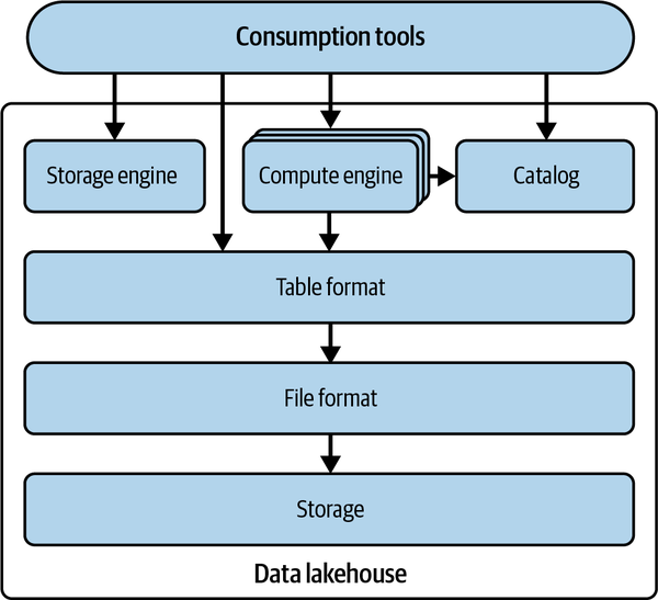
Figure 1-4. Technical components of a data lakehouse
To summarize, with modern innovations from the open standards previously discussed, the best of all worlds can exist by operating strictly on the data lake, and this architectural pattern is the data lakehouse. The key component that makes all this possible is the table format that enables engines to have the guarantees and improved performance over data lakes when working with data that just didn’t exist before. Now let’s turn the discussion to the Apache Iceberg table format.
What Is a Table Format?
A table format is a method of structuring a dataset’s files to present them as a unified “table.” From the user’s perspective, it can be defined as the answer to the question “what data is in this table?”
This simple answer enables multiple individuals, teams, and tools to interact with the data in the table concurrently, whether they are reading from it or writing to it. The main purpose of a table format is to provide an abstraction of the table to users and tools, making it easier for them to interact with the underlying data in an efficient manner.
Table formats have been around since the inception of RDBMSs such as System R, Multics, and Oracle, which first implemented Edgar Codd’s relational model, although the term table format was not used at that time. In these systems, users could refer to a set of data as a table, and the database engine was responsible for managing the dataset’s byte layout on disk in the form of files, while also handling complexities such as transactions.
All interactions with the data in these RDBMSs, such as reading and writing, are managed by the database’s storage engine. No other engine can interact with the files directly without risking system corruption. The details of how the data is stored are abstracted away, and users take for granted that the platform knows where the data for a specific table is located and how to access it.
However, in today’s big data world, relying on a single closed engine to manage all access to the underlying data is no longer practical. Your data needs access to a variety of compute engines optimized for different use cases such as BI or ML.
In a data lake, all your data is stored as files in some storage solution (e.g., Amazon S3, Azure Data Lake Storage [ADLS], Google Cloud Storage [GCS]), so a single table may be made of dozens, hundreds, thousands, or even millions of individual files on that storage. When using SQL with our favorite analytical tools or writing ad hoc scripts in languages such as Java, Scala, Python, and Rust, we wouldn’t want to constantly define which of these files are in the table and which of them aren’t. Not only would this be tedious, but it would also likely lead to inconsistency across different uses of the data.
So the solution was to create a standard method of understanding “what data is in this table” for data lakes, as illustrated in Figure 1-5.
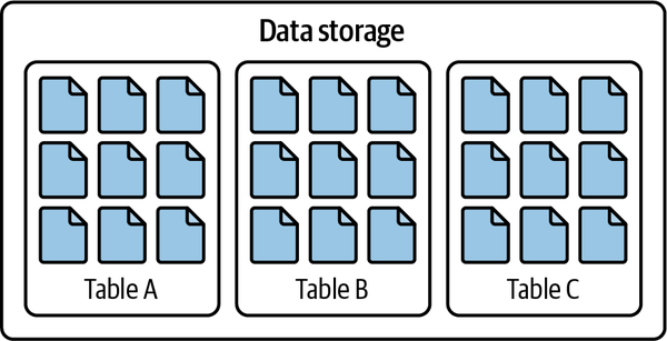
Figure 1-5. Datafiles organized into tables using a table format
Hive: The Original Table Format
When it came to the world of running analytics on Hadoop data lakes, the MapReduce framework was used, which required users to write complex and tedious Java jobs, which wasn’t accessible to many analysts. Facebook, feeling the pain of this situation, developed a framework called Hive in 2009. Hive provided a key benefit to make analytics on Hadoop much easier: the ability to write SQL instead of MapReduce jobs directly.
The Hive framework would take SQL statements and then convert them into MapReduce jobs that could be executed. To write SQL statements, there had to be a mechanism for understanding what data on your Hadoop storage represented a unique table, and the Hive table format and Hive Metastore for tracking these tables were born.
The Hive table format took the approach of defining a table as any and all files within a specified directory (or prefixes for object storage). The partitions of those tables would be the subdirectories. These directory paths defining the table are tracked by a service called the Hive Metastore, which query engines can access to know where to find the data applicable to their query. This is illustrated in Figure 1-6.
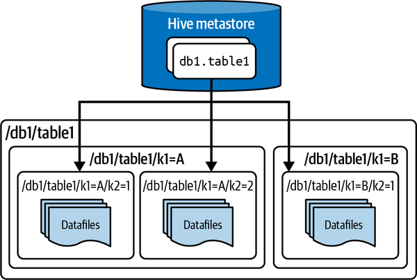
Figure 1-6. The architecture of a table stored using the Hive table format
The Hive table format had several benefits:
It enabled more efficient query patterns than full table scans, so techniques such as partitioning (dividing the data based on a partitioning key) and bucketing (an approach to partitioning or clustering/sorting that uses a hash function to evenly distribute values) made it possible to avoid scanning every file for faster queries.
It was file format agnostic, so it allowed the data community over time to develop better file formats, such as Apache Parquet, and use them in their Hive tables. It also did not require transformation prior to making the data available in a Hive table (e.g., Avro, CSV/TSV).
Through atomic swaps of the listed directory in the Hive Metastore, you can make all-or-nothing (atomic) changes to an individual partition in the table.
Over time, this became the de facto standard, working with most data tools and providing a uniform answer to “what data is in this table?”
While these benefits were significant, there were also many limitations that became apparent as time passed:
File-level changes are inefficient, since there was no mechanism to atomically swap a file in the same way the Hive Metastore could be used to swap a partition directory. You are essentially left making swaps at the partition level to update a single file atomically.
While you could atomically swap a partition, there wasn’t a mechanism for atomically updating multiple partitions as one transaction. This opens up the possibility for end users seeing inconsistent data between transactions updating multiple partitions.
There really aren’t good mechanisms to enable concurrent simultaneous updates, especially with tools beyond Hive itself.
An engine listing files and directories was time-consuming and slowed down queries. Having to read and list files and directories that may not need scanning in the resulting query comes at a cost.
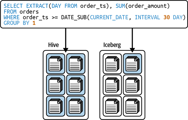
Partition columns were often derived from other columns, such as deriving a month column from a timestamp. Partitioning helped only if you filtered by the partition column, and someone who has a filter on the timestamp column may not intuitively know to also filter on the derived month column, leading to a full table scan since partitioning was not taken advantage of.
Table statistics would be gathered through asynchronous jobs, often resulting in state table statistics, if any statistics were available at all. This made it difficult for query engines to further optimize queries.
Since object storage often throttles requests against the same prefix (think of an object storage prefix as analogous to a file directory), queries on tables with large numbers of files in a single partition (so that all the files would be in one prefix) can have performance issues.
The larger the scale of the datasets and use cases, the more these problems would be amplified. This resulted in significant pain in need of a new solution, so newer table formats were created.
Modern Data Lake Table Formats
In seeking to address the limitations of the Hive table format, a new generation of table formats arose with different approaches in solving the problems with Hive.
Creators of modern table formats realized the flaw that led to challenges with the Hive table format was that the definition of the table was based on the contents of directories, not on the individual datafiles. Modern table formats such as Apache Iceberg, Apache Hudi, and Delta Lake all took this approach of defining tables as a canonical list of files, providing metadata for engines informing which files make up the table, not which directories. This more granular approach to defining “what is a table” unlocked the door to features such as ACID transactions, time travel, and more.
Modern table formats all aim to bring a core set of major benefits over the Hive table format:
They allow for ACID transactions, which are safe transactions that either complete in full or are canceled. In legacy formats such as the Hive table format, many transactions could not have these guarantees.
They enable safe transactions when there are multiple writers. If two or more writers write to a table, there is a mechanism to make sure the writer that completes their write second is aware of and considers what the other writer(s) have done to keep the data consistent.
They offer better collection of table statistics and metadata that can allow a query engine to plan scans more efficiently so that it will need to scan fewer files.
Let’s explore what Apache Iceberg is and how it came to be.
What Is Apache Iceberg?
Apache Iceberg is a table format created in 2017 by Netflix’s Ryan Blue and Daniel Weeks. It arose from the need to overcome challenges with performance, consistency, and many of the challenges previously stated with the Hive table format. In 2018, the project was made open source and was donated to the Apache Software Foundation, where many other organizations started getting involved with it, including Apple, Dremio, AWS, Tencent, LinkedIn, and Stripe. Many additional organizations have contributed to the project since then.
How Apache Iceberg Came to Be
Netflix, in the creation of what became the Apache Iceberg format, concluded that many of the problems with the Hive format stemmed from one simple but fundamental flaw: each table is tracked as directories and subdirectories, limiting the granularity that is necessary to provide consistency guarantees, better concurrency, and several of the features that often are available in data warehouses.
With this in mind, Netflix set out to create a new table format with several goals in mind:
- Consistency
If updates to a table occur over multiple partitions, it must not be possible for end users to experience inconsistency in the data they are viewing. An update to a table across multiple partitions should be done quickly and atomically so that the data is consistent to end users. They see the data either before the update or after the update, and not in between.
- Performance
With Hive’s file/directory listing bottleneck, query planning would take excessively long to complete before actually executing the query. The table should provide metadata and avoid excessive file listing so that not only can query planning be a faster process, but also the resulting plans can be executed more quickly since they scan only the files necessary to satisfy the query.
- Easy to use
To get the benefits of techniques such as partitioning, end users should not have to be aware of the physical structure of the table. The table should be able to give users the benefits of partitioning based on naturally intuitive queries and not depend on filtering extra partition columns derived from a column they are already filtering by (e.g., filtering by a month column when you’ve already filtered the timestamp it is derived from).
- Evolvability
Updating schemas of Hive tables could result in unsafe transactions, and updating how a table is partitioned would result in a need to rewrite the entire table. A table should be able to evolve its schema and partitioning scheme safely and without the need for rewriting.
- Scalability
All the preceding goals should be able to be accomplished at the petabyte scale of Netflix’s data.
So the team began creating the Iceberg format, which focuses on defining a table as a canonical list of files instead of tracking a table as a list of directories and subdirectories. The Apache Iceberg project is a specification, or a standard of how metadata defining a data lakehouse table should be written across several files. To support the adoption of this standard, Apache Iceberg has many support libraries to help individuals work with the format or compute engines to implement support. Along with these libraries, the project has created implementations for open source compute engines such as Apache Spark and Apache Flink.
Apache Iceberg aims for existing tools to embrace the standard and is designed to take advantage of existing, popular storage solutions and compute engines in the hope that existing options will support working with the standard. The purpose of this approach is to let the ecosystem of existing data tools build out support for Apache Iceberg tables and let Iceberg become the standard for how engines can recognize and work with tables on the data lake. The goal is for Apache Iceberg to become so ubiquitous in the ecosystem that it becomes another implementation detail that many users don’t have to think about. They just know they are working with tables and don’t need to think about it beyond that, regardless of which tool they are using to interact with the table. This is already becoming a reality as many tools allow end users to work with Apache Iceberg tables so easily that they don’t need to understand the underlying Iceberg format. Eventually, with automated table optimization and ingestion tools, even more technical users such as data engineers won’t have to think as much about the underlying format and will be able to work with their data lake storage in the way they’ve worked with data warehouses, without ever dealing directly with the storage layer.
The Apache Iceberg Architecture
Apache Iceberg tracks a table’s partitioning, sorting, schema over time, and so much more using a tree of metadata that an engine can use to plan queries at a fraction of the time it would take with legacy data lake patterns. Figure 1-7 depicts this tree of metadata.
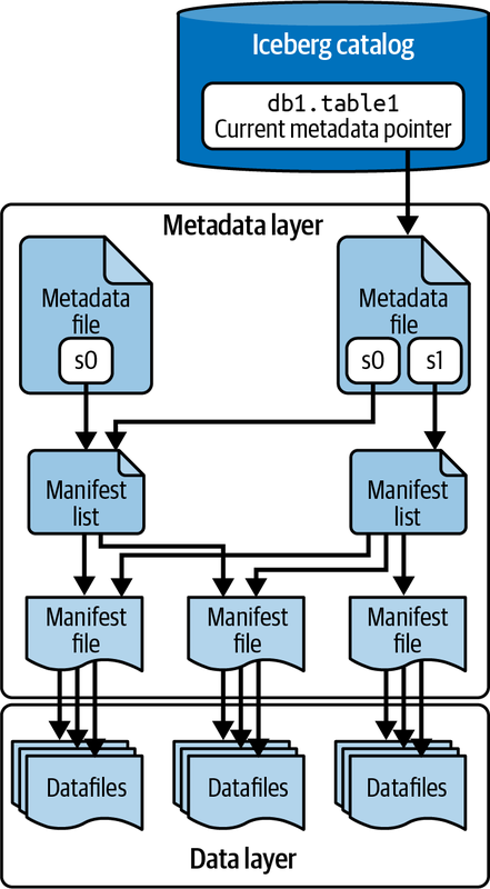
Figure 1-7. The Apache Iceberg architecture
This metadata tree breaks down the metadata of the table into four components:
- Manifest file
A list of datafiles, containing each datafile’s location/path and key metadata about those datafiles, which allows for creating more efficient execution plans.
- Manifest list
Files that define a single snapshot of the table as a list of manifest files along with stats on those manifests that allow for creating more efficient execution plans.
- Metadata file
Files that define a table’s structure, including its schema, partitioning scheme, and a listing of snapshots.
- Catalog
Tracks the table location (similar to the Hive Metastore), but instead of containing a mapping of table name -> set of directories, it contains a mapping of table name -> location of the table’s most recent metadata file. Several tools, including a Hive Metastore, can be used as a catalog, and we have dedicated Chapter 5 to this subject.
Each of these files will be covered in more depth in Chapter 2.
Key Features of Apache Iceberg
Apache Iceberg’s unique architecture enables an ever-growing number of features that go beyond just solving the challenges with Hive and instead unlock entirely new functionality for data lakes and data lakehouse workloads. In this section, we provide a high-level overview of key features of Apache Iceberg. We’ll go into more depth on these features in later chapters.
ACID transactions
Apache Iceberg uses optimistic concurrency control to enable ACID guarantees, even when you have transactions being handled by multiple readers and writers. Optimistic concurrency assumes transactions won’t conflict and checks for conflicts only when necessary, aiming to minimize locking and improve performance. This way, you can run transactions on your data lakehouse that either commit or fail and nothing in between. A pessimistic concurrency model, which uses locks to prevent conflicts between transactions, assuming conflicts are likely to occur, was unavailable in Apache Iceberg at the time of this writing but may be coming in the future.
Concurrency guarantees are handled by the catalog, as it is typically a mechanism that has built-in ACID guarantees. This is what allows transactions on Iceberg tables to be atomic and provide correctness guarantees. If this didn’t exist, two different systems could have conflicting updates, resulting in data loss.
Partition evolution
A big headache with data lakes prior to Apache Iceberg was dealing with the need to change the table’s physical optimization. Too often, when your partitioning needs to change, the only choice you have is to rewrite the entire table, and at scale this can get very expensive. The alternative is to just live with the existing partitioning scheme and sacrifice the performance improvements a better partitioning scheme can provide.
With Apache Iceberg you can update how the table is partitioned at any time without the need to rewrite the table and all its data. Since partitioning has everything to do with the metadata, the operations needed to make this change to your table’s structure are quick and cheap.
Figure 1-8 depicts a table that was initially partitioned by month and then evolved to partition based on day going forward. The previously written data remains in month partitions while new data is written in day partitions, and in a query, the engine makes a plan for each partition based on the partition scheme applied to it.
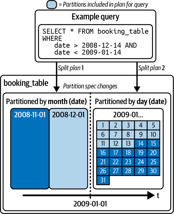
Figure 1-8. Partition evolution
Row-level table operations
You can optimize the table’s row-level update patterns to take one of two forms: copy-on-write (COW) or merge-on-read (MOR). When using COW, for a change of any row in a given datafile, the entire file is rewritten (with the row-level change made in the new file) even if a single record in it is updated. When using MOR, for any row-level updates, only a new file that contains the changes to the affected row that is reconciled on reads is written. This gives flexibility to speed up heavy update and delete workloads.
Time travel
Apache Iceberg provides immutable snapshots, so the information for the table’s historical state is accessible, allowing you to run queries on the state of the table at a given point in time in the past, or what’s commonly known as time travel. This can help you in situations such as doing end-of-quarter reporting without the need for duplicating the table’s data to a separate location or for reproducing the output of an ML model as of a certain point in time. This is depicted in Figure 1-10.
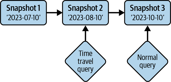
Figure 1-10. Querying the table as it was using time travel
Version rollback
Not only does Iceberg’s snapshot isolation allow you to query the data as it is, but it also reverts the table’s current state to any of those previous snapshots. Therefore, undoing mistakes is as easy as rolling back (see Figure 1-11).
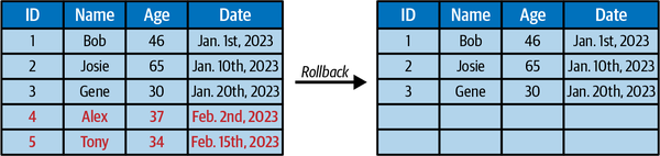
Figure 1-11. Moving the table’s state to a previous point in time by rolling back
Schema evolution
Tables change, whether that means adding/removing a column, renaming a column, or changing a column’s data type. Regardless of how your table needs to evolve, Apache Iceberg gives you robust schema evolution features—for example, updating an int column to a long column as values in the column get larger.
Conclusion
In this chapter, you learned that Apache Iceberg is a data lakehouse table format built to improve upon many of the areas where Hive tables were lacking. By decoupling from relying on the physical structure of files along with its multilevel metadata tree, Iceberg is able to provide Hive transactions, ACID guarantees, schema evolution, partition evolution, and several other features enabling the data lakehouse. The Apache Iceberg project is able to do this by building a specification and supporting libraries that let existing data tools build support for the open table format.
In Chapter 2, we’ll take a deep dive into Apache Iceberg’s architecture that makes all this possible.
Get Apache Iceberg: The Definitive Guide now with the O’Reilly learning platform.
O’Reilly members experience books, live events, courses curated by job role, and more from O’Reilly and nearly 200 top publishers.

