Amazon Redshift: The Definitive Guide

Chapter 4. Data Transformation Strategies

A recent report published by Forbes describes how some stockbrokers and trading firms were able to access and analyze data faster than their competitors. This allowed them to “execute trades at the best price, microseconds ahead of the crowd. The win was ever so slight in terms of time, but massive in terms of the competitive advantage gained by speed to insight.”

When considering an analytics solution, speed to insights is important and the quicker an organization can respond to a shift in their data, the more competitive they will be. In many cases, to get the insights you need, the data needs to be transformed. As briefly discussed in Chapter 3, “Setting Up Your Data Models and Ingesting Data”, you can use an ETL approach, which reads the source data, processes the transformations in an external application, and loads the results, or you can use an ELT approach, which uses the data you just loaded and transforms the data in-place using the power of the Amazon Redshift compute.

In this chapter, we’ll start by “Comparing ELT and ETL Strategies” to help you decide which data loading strategy to use when building your data warehouse. We’ll also dive deep into some of the unique features of Redshift that were built for analytics use cases and that empower “In-Database Transformation” as well as how you can leverage in-built “Scheduling and Orchestration” capabilities to run your pipelines. Then we’ll cover how Amazon Redshift takes the ELT strategy even further, by allowing you to “Access All Your Data” even if it was not loaded into Redshift. Finally, we’ll cover when it may make sense to use an “External Transformation” strategy and how to use AWS Glue Studio to build your ETL pipelines.

Comparing ELT and ETL Strategies

Regardless of an ELT or ETL strategy, each can support the common goals of your data management platform, which typically involve cleansing, transforming, and aggregating the data for loading into your reporting data model. These are all resource-intensive operations, and the primary difference between the two strategies is where the processing happens: in the compute of your ETL server(s) or in the compute of your data warehouse platform. ETL processes involve reading data from multiple sources and transforming the data using the functions and capabilities of the ETL engine. In contrast, ELT processes also involve extracting data from various sources but first loading it into the data warehouse. The transformation step is performed after the data has been loaded using familiar SQL semantics. Some things to consider when choosing between the two include:

Performance and scalability

ETL processes are dependent on the resources of the ETL server(s) and require platform owners to correctly manage and size the environment. Compute platforms like Spark can be used to parallelize the data transformations and AWS Glue is provided as a serverless option for managing ETL pipelines. ELT processing is performed using the compute resources of the data warehouse. In the case of Amazon Redshift, the power of the MPP architecture is used to perform the transformations. Historically, transforming the data externally was preferred because the processing is offloaded to independent compute. However, modern data warehouse platforms, including Amazon Redshift, scale dynamically and can support mixed workloads, making an ELT strategy more attractive. In addition, since data warehouse platforms are designed to process and transform massive quantities of data using native database functions, ELT jobs tend to perform better. Finally, ELT strategies are free from network bottlenecks, which are required with ETL to move data in and out for processing.

Flexibility

While any transformation code in your data platform should follow a development lifecycle, with an ETL strategy, the code is typically managed by a team with specialized skill in an external application. In contrast, with an ELT strategy, all of your raw data is available to query and transform in the data management platform. Analysts can write code using familiar SQL functions leveraging the skills they already have. Empowering analysts shortens the development lifecycle because they can prototype the code and validate the business logic. The data platform owners would be responsible for optimizing and scheduling the code.

Metadata management and orchestration

One important consideration for your data strategy is how to manage job metadata and orchestration. Leveraging an ELT strategy means that the data platform owner needs to keep track of the jobs, their dependencies, and load schedules. ETL tools typically have capabilities that capture and organize metadata about sources, targets, and job characteristics as well as data lineage. They also can orchestrate jobs and build dependencies across multiple data platforms.

Ultimately, the choice between ETL and ELT will depend on the specific needs of the analytics workload. Both strategies have strengths and weaknesses, and the decision of which you use depends on the characteristics of the data sources, the transformation requirements, and the performance and scalability needs of the project. To mitigate the challenges with each, many users take a hybrid approach. You can take advantage of the metadata management and orchestration capabilities of ETL tools as well as the performance and scalability of ELT processing by building jobs that translate the ETL code to SQL statements. In “External Transformation”, we will discuss in more detail how this is possible.

In-Database Transformation

With the variety and velocity of data present today, the challenge of designing a data platform is to make it both scalable and flexible. Amazon Redshift continues to innovate and provide functionality to process all your data in one place with its in-database transformation (ELT) capabilities. Being an ANSI SQL compatible relational database, Amazon Redshift supports SQL commands, making it a familiar development environment for most database developers. Amazon Redshift also supports advanced functions present in modern data platforms such as Window Functions, HyperLogLog Functions, and Recursive CTE (common table expressions), to name a few. In addition to those functions you may be familiar with, Amazon Redshift supports unique capabilities for analytical processing. For example, Amazon Redshift supports in-place querying for “Semistructured Data”, providing analysts a way to access this data in a performant way and without waiting for it to be loaded into tables and columns. In addition, if you need to extend the capabilities of Amazon Redshift, you can leverage “User-Defined Functions” that can run inside the database or call external services. Finally, “Stored Procedures” allow you to package your transformation logic. They can return a result set given input parameters or even perform data loading and managed operations like loading a fact, dimension, or aggregate table.

Semistructured Data

Semistructured data falls under the category of data that doesn’t conform to a rigid schema expected in relational databases. Semistructured formats are common and often preferred in web logs, sensor data, or API messages because these applications often have to send data with nested relationships, and rather than making multiple round-trips, it is more efficient to send the data once. Semistructured data contains complex values such as arrays and nested structures that are associated with serialization formats, such as JSON. While there are third-party tools you can use to transform your data outside the database, it would require engineering resources to build and maintain that code and may not be as performant. Whether you are accessing “External Amazon S3 Data” or locally loaded data, Amazon Redshift leverages the PartiQL syntax for analyzing and transforming semistructured data. A special data type, SUPER, was launched to store this data in its native form. However, when accessed from Amazon S3, it will be cataloged with a data type of struct or array.

In the following example, we’re referencing a file that has landed in an Amazon S3 environment. You can catalog this file and make it accessible in Amazon Redshift by creating an external schema and mapping any file that exists in this Amazon S3 prefix to this table definition.

The first query (Example 4-1) finds the total sales revenue per event.

Example 4-1. Create external table from JSON data

CREATE external SCHEMA IF NOT EXISTS nested_json
FROM data catalog DATABASE 'nested_json'
IAM_ROLE default
CREATE EXTERNAL DATABASE IF NOT EXISTS;

DROP TABLE IF EXISTS nested_json.nested_json;
CREATE EXTERNAL TABLE nested_json.nested_json (
    c_name varchar,
    c_address varchar,
    c_nationkey int,
    c_phone varchar,
    c_acctbal float,
    c_mktsegment varchar,
    c_comment varchar,
    orders struct<"order":array<struct<
      o_orderstatus:varchar,
      o_totalprice:float,
      o_orderdate:varchar,
      o_order_priority:varchar,
      o_clerk:varchar,
      o_ship_priority:int,
      o_comment:varchar
      >>> )
row format serde 'org.openx.data.jsonserde.JsonSerDe'
with serdeproperties ('paths'='c_name,c_address,c_nationkey,c_phone,
  c_acctbal,c_mktsegment,c_comment,Orders')
stored as inputformat 'org.apache.hadoop.mapred.TextInputFormat'
outputformat 'org.apache.hadoop.hive.ql.io.HiveIgnoreKeyTextOutputFormat'
location 's3://redshift-immersionday-labs/data/nested-json/';

This data file is located in the us-west-2 region, and this example will work only if your Amazon Redshift data warehouse is also in that region. Also, we’ve referenced the default IAM role. Be sure to modify the role to allow read access to this Amazon S3 location as well as to have access to manage the AWS Glue Data Catalog.

Now that the table is available, it can be queried and you can access top-level attributes without any special processing (Example 4-2).

Example 4-2. Top-level attributes

SELECT cust.c_name,
  cust.c_nationkey,
  cust.c_address
FROM nested_json.nested_json cust
WHERE cust.c_nationkey = '-2015'
  AND cust.c_address like '%E12';

Using the PartiQL syntax, you can access the nested struct data. In Example 4-3, we are un-nesting the data in the orders field and showing the multiple orders associated to the customer record.

Example 4-3. Un-nested attributes (external)

SELECT cust.c_name,
   cust_order.o_orderstatus,
   cust_order.o_totalprice,
   cust_order.o_orderdate::date,
   cust_order.o_order_priority,
   cust_order.o_clerk,
   cust_order.o_ship_priority,
   cust_order.o_comment
FROM nested_json.nested_json cust,
     cust.orders.order cust_order
WHERE cust.c_nationkey = '-2015'
  AND cust.c_address like '%E12';

In addition to accessing data in S3, this semistructured data can be loaded into your Amazon Redshift table using the SUPER data type. In Example 4-4, this same file is loaded into a physical table. One notable difference when loading into Amazon Redshift is that no information about the schema of the orders column mapped to the SUPER data type is required. This simplifies the loading and metadata management process as well as provides flexibility in case of metadata changes.

Example 4-4. Create local table from JSON data

DROP TABLE IF EXISTS nested_json_local;
CREATE TABLE nested_json_local (
    c_name varchar,
    c_address varchar,
    c_nationkey int,
    c_phone varchar,
    c_acctbal float,
    c_mktsegment varchar,
    c_comment varchar,
    orders SUPER);

COPY nested_json_local
from 's3://redshift-immersionday-labs/data/nested-json/'
IAM_ROLE default REGION 'us-west-2'
JSON 'auto ignorecase';

We’ve referenced the default IAM role. Be sure to modify the role to grant access to read from this Amazon S3 location.

Now that the table is available, it can be queried. Using the same PartiQL syntax, you can access the order details (Example 4-5).

Example 4-5. Unnested attributes (local)

SET enable_case_sensitive_identifier TO true;
SELECT cust.c_name,
   cust_order.o_orderstatus,
   cust_order.o_totalprice,
   cust_order.o_orderdate::date,
   cust_order.o_order_priority,
   cust_order.o_clerk,
   cust_order.o_ship_priority,
   cust_order.o_comment
FROM nested_json_local cust,
     cust.orders."Order" cust_order
WHERE cust.c_nationkey = '-2015'
  AND cust.c_address like '%E12';

The enable_case_sensitive_identifier is an important parameter when querying SUPER data if your input has mixed case identifiers. For more information, see the online documentation.

For more details and examples on querying semistructured data, see the online documentation.

User-Defined Functions

If a built-in function is not available for your specific transformation needs, Amazon Redshift has a few options for extending the functionality of the platform. Amazon Redshift allows you to create scalar user-defined functions (UDFs) in three flavors: SQL, Python, and Lambda. For detailed documentation on creating each of these types of functions, see the online documentation.

A scalar function will return exactly one value per invocation. In most cases, you can think of this as returning one value per row.

An SQL UDF leverages existing SQL syntax. It can be used to ensure consistent logic is applied and to simplify the amount of code each user would have to write individually. In Example 4-6, from the Amazon Redshift UDFs GitHub Repo, you’ll see an SQL function that takes two input parameters; the first varchar field is the data to be masked, and the second field is the classification of the data. The result is a different masking strategy based on the data classification.

Example 4-6. SQL UDF definition

CREATE OR REPLACE function f_mask_varchar (varchar, varchar)
  returns varchar
immutable
AS $$
  SELECT case $2
    WHEN 'ssn' then
      substring($1, 1, 7)||'xxxx'
    WHEN 'email' then
      substring(SPLIT_PART($1, '@', 1), 1, 3) + 'xxxx@' + SPLIT_PART($1, '@', 2)
    ELSE substring($1, 1, 3)||'xxxxx' end
$$ language sql;

Users can reference an SQL UDF within a SELECT statement. In this scenario, you might write the SELECT statement as shown in Example 4-7.

Example 4-7. SQL UDF access

DROP TABLE IF EXISTS customer_sqludf;
CREATE TABLE customer_sqludf (cust_name varchar, email varchar, ssn varchar);
INSERT INTO customer_sqludf VALUES('Jane Doe', '[e-mail]', '123-45-6789');

SELECT
 f_mask_varchar (cust_name, NULL) mask_name, cust_name,
 f_mask_varchar (email, 'email') mask_email, email,
 f_mask_varchar (ssn, 'ssn') mask_ssn, ssn
FROM customer_sqludf;

The SELECT statement in Example 4-7 results in the following output:

mask_name	name	mask_email	email	mask_ssn	ssn
Janxxxxx	Jane Doe	[e-mail]	[e-mail]	123-45-xxxx	123-45-6789

A Python UDF allows users to leverage Python code to transform their data. In addition to core Python libraries, users can import their own libraries to extend the functionality available in Amazon Redshift. In Example 4-8, from the Amazon Redshift UDFs GitHub Repo, you’ll see a Python function that leverages an external library, ua_parser, which can parse a user-agent string into a JSON object and return the client OS family. Please refer to the GitHub Repo for detailed instructions on how to install this example.

Example 4-8. Python UDF definition

CREATE OR REPLACE FUNCTION f_ua_parser_family (ua VARCHAR)
RETURNS VARCHAR IMMUTABLE AS $$
  FROM ua_parser import user_agent_parser
  RETURN user_agent_parser.ParseUserAgent(ua)['family']
$$ LANGUAGE plpythonu;

Similar to SQL UDFs, users can reference a Python UDF within a SELECT statement. In this example, you might write the SELECT statement shown in Example 4-9.

Example 4-9. Python UDF access

SELECT f_ua_parser_family (agent) family, agent FROM weblog;

The SELECT statement in Example 4-9 results in the following output:

family	agent
Chrome	Mozilla/5.0 (Macintosh; Intel Mac OS X 10_9_4) AppleWebKit/537.36 (KHTML, like Gecko) Chrome/41.0.2272.104 Safari/537.36

Lastly, the Lambda UDF allows users to interact and integrate with external components outside of Amazon Redshift. You can write Lambda UDFs in any supported programming language, such as Java, Go PowerShell, Node.js, C#, Python, Ruby, or a custom runtime. This functionality enables new Amazon Redshift use cases, including data enrichment from external data stores (e.g., Amazon DynamoDB, Amazon ElastiCache, etc.), data enrichment from external APIs (e.g., Melissa Global Address Web API, etc.), data masking and tokenization from external providers (e.g., Protegrity), and conversion of legacy UDFs written in other languages such as C, C++, and Java. In Example 4-10, from the Amazon Redshift UDFs GitHub Repo, you’ll see a Lambda function that leverages the AWS Key Management Service (KMS) and takes an incoming string to return the encrypted value. The first code block establishes a Lambda function, f-kms-encrypt, which expects a nested array of arguments passed to the function. In this example, the user would supply the kmskeyid and the columnValue as input parameters; argument[0] and argument[1]. The function will use the boto3 library to call the kms service to return the encrypted response. Please refer to the GitHub Repo for detailed instructions on how to install this example.

Example 4-10. Lambda function definition

import json, boto3, os, base64
kms = boto3.client('kms')
def handler(event, context):
  ret = dict()
  res = []
  for argument in event['arguments']:
    try:
      kmskeyid = argument[0]
      columnValue = argument[1]
      if (columnValue == None):
          response = None
      else:
          ciphertext = kms.encrypt(KeyId=kmskeyid, Plaintext=columnValue)
          cipherblob = ciphertext["CiphertextBlob"]
          response = base64.b64encode(cipherblob).decode('utf-8')
      res.append(response)
    except Exception as e:
      print (str(e))
      res.append(None)
  ret['success'] = True
  ret['results'] = res
  return json.dumps(ret)

The next code block establishes the Amazon Redshift UDF, which references the Lambda function (Example 4-11).

Example 4-11. Lambda UDF definition

CREATE OR REPLACE EXTERNAL FUNCTION f_kms_encrypt (key varchar, value varchar)
RETURNS varchar(max) STABLE
LAMBDA 'f-kms-encrypt'
IAM_ROLE default;

We’ve referenced the default IAM role. Be sure to modify the role to grant access to execute the Lambda function created previously.

Just like the SQL and Python UDFs, users can reference a Lambda UDF within a SELECT statement. In this scenario, you might write the SELECT statement show in Example 4-12.

Example 4-12. Lambda UDF access

SELECT f_kms_encrypt (email) email_encrypt, email FROM customer;

The SELECT statement in Example 4-12 results in the following output:

email_encrypt	email
AQICAHiQbIJ478Gbu8DZyl0frUxOrbgDlP+CyfuWCuF0kHJyWg …​	[e-mail]

For more details on Python UDFs, see the “Introduction to Python UDFs in Amazon Redshift” blog post, and for more details on Lambda UDFs, see the “Accessing External Components Using Amazon Redshift Lambda UDFs” blog post.

Stored Procedures

An Amazon Redshift stored procedure is a user-created object to perform a set of SQL queries and logical operations. The procedure is stored in the database and is available to users who have privileges to execute it. Unlike a scalar UDF function, which can operate on only one row of data in a table, a stored procedure can incorporate data definition language (DDL) and data manipulation language (DML) in addition to SELECT queries. Also, a stored procedure doesn’t have to return a value and can contain looping and conditional expressions.

Stored procedures are commonly used to encapsulate logic for data transformation, data validation, and business-specific operations as an alternative to shell scripting, or complex ETL and orchestration tools. Stored procedures allow the ETL/ELT logical steps to be fully enclosed in a procedure. You may write the procedure to commit data incrementally or so that it either succeeds completely (processes all rows) or fails completely (processes no rows). Because all the processing occurs on the data warehouse, there is no overhead to move data across the network and you can take advantage of Amazon Redshift’s ability to perform bulk operations on large quantities of data quickly because of its MPP architecture.

In addition, because stored procedures are implemented in the PL/pgSQL programming language, you may not need to learn a new programming language to use them. In fact, you may have existing stored procedures in your legacy data platform that can be migrated to Amazon Redshift with minimal code changes. Re-creating the logic of your existing processes using an external programming language or a new ETL platform could be a large project. AWS also provides the AWS Schema Conversion Tool (SCT), a migration assistant that can help by converting existing code in other database programming languages to Amazon Redshift native PL/pgSQL code.

In Example 4-13, you can see a simple procedure that will load data into a staging table from Amazon S3 and load new records into the lineitem table, while ensuring that duplicates are deleted. This procedure takes advantage of the MERGE operator and can accomplish the task using one statement. In this example, there are constant variables for the l_orderyear and l_ordermonth. However, this can be easily made dynamic using the date_part function and current_date variable to determine the current year and month to load or by passing in a year and month parameter to the procedure.

Example 4-13. Stored procedure definition

CREATE TABLE IF NOT EXISTS lineitem (
  L_ORDERKEY varchar(20) NOT NULL,
  L_PARTKEY varchar(20),
  L_SUPPKEY varchar(20),
  L_LINENUMBER integer NOT NULL,
  L_QUANTITY varchar(20),
  L_EXTENDEDPRICE varchar(20),
  L_DISCOUNT varchar(20),
  L_TAX varchar(20),
  L_RETURNFLAG varchar(1),
  L_LINESTATUS varchar(1),
  L_SHIPDATE date,
  L_COMMITDATE date,
  L_RECEIPTDATE date,
  L_SHIPINSTRUCT varchar(25),
  L_SHIPMODE varchar(10),
  L_COMMENT varchar(44));

CREATE TABLE stage_lineitem (LIKE lineitem);

CREATE OR REPLACE PROCEDURE lineitem_incremental()
AS $$
DECLARE
  yr CONSTANT INTEGER := 1998; --date_part('year',current_date);
  mon CONSTANT INTEGER := 8; --date_part('month', current_date);
  query VARCHAR;
BEGIN
  TRUNCATE stage_lineitem;
  query := 'COPY stage_lineitem ' ||
  	'FROM ''s3://redshift-immersionday-labs/data/lineitem-part/' ||
	  'l_orderyear=' || yr || '/l_ordermonth=' || mon || '/''' ||
    ' IAM_ROLE default REGION ''us-west-2'' gzip delimiter ''|''';
  EXECUTE query;

  MERGE INTO lineitem
  USING stage_lineitem s ON s.l_orderkey=lineitem.l_orderkey
  AND s.l_linenumber = lineitem.l_linenumber
  WHEN MATCHED THEN DELETE
  WHEN NOT MATCHED THEN INSERT
    VALUES ( s.L_ORDERKEY, s.L_PARTKEY, s.L_SUPPKEY, s.L_LINENUMBER,
      s.L_QUANTITY, s.L_EXTENDEDPRICE, s.L_DISCOUNT, s.L_TAX,
      s.L_RETURNFLAG, s.L_LINESTATUS, s.L_SHIPDATE, s.L_COMMITDATE,
      s.L_RECEIPTDATE, s.L_SHIPINSTRUCT, s.L_SHIPMODE, s.L_COMMENT);

END;
$$ LANGUAGE plpgsql;

We’ve referenced the default IAM role. Be sure to modify the role to grant access to read from this Amazon S3 location.

You can execute a stored procedure by using the call keyword (Example 4-14).

Example 4-14. Stored procedure access

CALL lineitem_incremental();

For more details on Amazon Redshift stored procedures, see the “Bringing Your Stored Procedures to Amazon Redshift” blog post.

Scheduling and Orchestration

When you start to think about orchestrating your data pipeline, you want to consider the complexity of the workflow and the dependencies on external processes. Some users have to manage multiple systems with complex dependencies. You may have advanced notification requirements if a job fails or misses an SLA. If so, you may consider a third-party scheduling tool. Popular third-party enterprise job scheduling tools include Tivoli, Control-M, and AutoSys, which each have integrations with Amazon Redshift allowing you to initiate a connection and execute one or multiple SQL statements. AWS also offers the Amazon Managed Workflow orchestration for Apache Airflow (MWAA) service, which is based on the open source Apache Airflow project. This can be useful if you are already running an Apache Airflow workflow and would like to migrate it to the cloud.

However, if you can trigger your loads based on time-based triggers, you can leverage the query scheduler. When you’re using the query scheduler, the UI will leverage the foundational services of the Amazon Redshift Data API and EventBridge.

To use the query scheduler to trigger simple time-based queries, navigate to the Query Editor V2, prepare your query, and click the Schedule button (Figure 4-1). For this example, we will use a COPY statement to load the stage_lineitem table.

Set the connection (Figure 4-2) as well as the IAM role the scheduler will assume to execute the query. In the subsequent dialog, select the applicable Amazon Redshift data warehouse from the list and the corresponding account and region. In our case, we will use “Temporary credentials” to connect. See Chapter 2, “Getting Started with Amazon Redshift” for more details on other connection strategies.

Figure 4-1. Schedule button

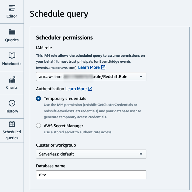
Figure 4-2. Choose connection

Next, set the query name that will be executed and the optional description (Figure 4-3). The query will be copied over from the editor page.

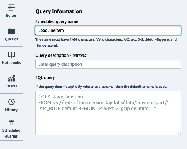
Figure 4-3. Set query

Next, set the time-based schedule either in Cron format or by selecting the applicable radio options (Figure 4-4). Optionally, choose if you’d like execution events to be delivered to an Amazon Simple Notification Service (SNS) topic so you can receive notifications. Click Save Changes to save the schedule.

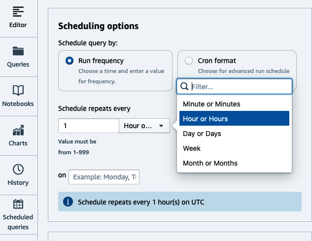
Figure 4-4. Set schedule

To see the list of scheduled queries, navigate to the Scheduled queries page of the Query Editor V2 (Figure 4-5).

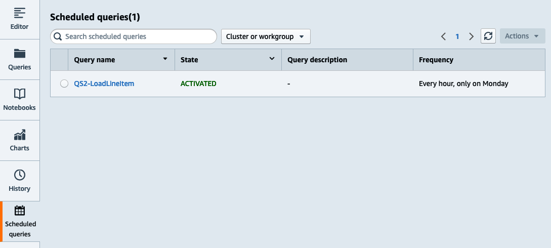
Figure 4-5. List scheduled queries

To manage the scheduled job, click on the scheduled query. In this screen you can modify the job, deactivate it, or delete it. You can also inspect the history, which contains the start/stop time as well as the job status (see Figure 4-6).

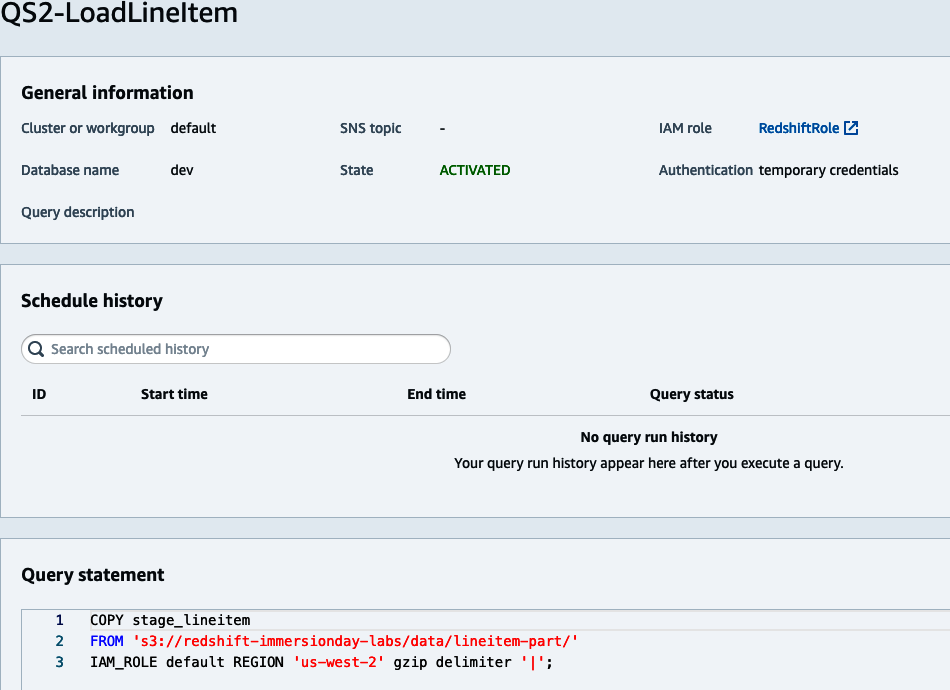
Figure 4-6. See schedule history

You can also see the resources created in EventBridge. Navigate to the EventBridge Rules page and notice a new Scheduled rule was created (Figure 4-7).

Figure 4-7. Scheduled rule

Inspecting the rule target (Figure 4-8), you will see Redshift cluster target type along with the parameter needed to execute the query.

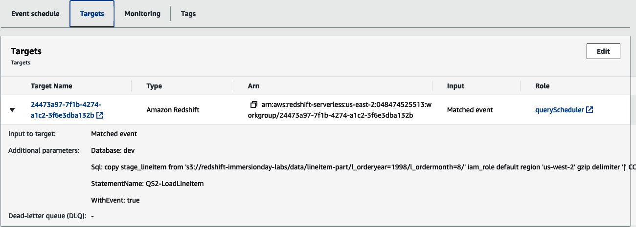
Figure 4-8. Scheduled rule target

Access All Your Data

To complete the ELT story, Amazon Redshift supports access to data even if it was not loaded. The Amazon Redshift compute will process your data using all the transformation capabilities already mentioned without the need of a separate server for processing. Whether it is “External Amazon S3 Data”, “External Operational Data”, or even “External Amazon Redshift Data”, queries are submitted in your Amazon Redshift data warehouse using familiar ANSI SQL syntax; only the applicable data is processed by the Amazon Redshift compute. It can be joined to local data and used to populate tables local to your Amazon Redshift data warehouse.

External Amazon S3 Data

Amazon Redshift enables you to read and write external data that is stored in Amazon S3 using simple SQL queries. Accessing data on Amazon S3 enhances the interoperability of your data because you can access the same Amazon S3 data from multiple compute platforms beyond Amazon Redshift. Such platforms include Amazon Athena, Amazon EMR, Presto, and any other compute platform that can access Amazon S3. Using this feature Amazon Redshift can join external Amazon S3 tables with tables that reside on the local disk of your Amazon Redshift data warehouse. When using a provisioned cluster, Amazon Redshift will leverage a fleet of nodes called Amazon Redshift Spectrum, which further isolates the Amazon S3 processing and applies optimizations like predicate pushdown and aggregation to the Amazon Redshift Spectrum compute layer, improving query performance. Types of predicate operators you can push to Amazon Redshift Spectrum include: =, LIKE, IS NULL, and CASE WHEN. In addition, you can employ transformation logic where many aggregation and string functions are pushed to the Amazon Redshift Spectrum layer. Types of aggregate functions include: COUNT, SUM, AVG, MIN, and MAX.

Amazon Redshift Spectrum processes Amazon S3 data using compute up to 10 times the number of slices in your provisioned cluster. It also comes with a cost of $5/TB scanned. In contrast, when you query Amazon S3 data using Amazon Redshift serverless, the processing occurs on your Amazon Redshift compute and the cost is part of RPU pricing.

Querying external Amazon S3 data works by leveraging an external metadata catalog that organizes datasets into databases and tables. You then map a database to an Amazon Redshift schema and provide credentials via an IAM ROLE, which determines what level of access you have. In Example 4-15, your metadata catalog is the AWS Glue data catalog, which contains a database called externaldb. If that database doesn’t exist, this command will create it. We’ve mapped that database to a new schema, externalschema, using the default IAM role attached to the data warehouse. In addition to the AWS Glue data catalog, users may map to a hive metastore if your data is located in an EMR cluster or in a self-managed Apache Hadoop environment. For more details on options when creating external schema, see the online documentation.

Example 4-15. Create external S3 schema

CREATE EXTERNAL SCHEMA IF NOT EXISTS externalschema
FROM data catalog DATABASE 'externaldb'
IAM_ROLE default
CREATE EXTERNAL DATABASE IF NOT EXISTS;

We’ve referenced the default IAM role. Be sure to modify the role to have access to manage the AWS Glue Data Catalog.

Once the external schema is created, you can easily query the data similar to a table that was loaded into Amazon Redshift. In Example 4-16, you can query data from your external table joined with data that is stored locally. Please note, the data sets referenced in the below example have not been setup. The query provided is for illustrative purposes only.

Example 4-16. External S3 table access

SELECT
 t.returnflag,
 t.linestatus,
 c.zip,
 sum(t.quantity) AS sum_qty,
 sum(t.extendedprice*(1-t.discount)*(1+t.tax)) AS sum_charge
FROM externalschema.transactions t
JOIN public.customers c on c.id = t.customer_id
WHERE t.year = 2022 AND t.month = 1
GROUP BY t.returnflag, t.linestatus, c.zip;

This query has a filter that restricts the data from the external table to January 2022 and a simple aggregation. When using a provisioned cluster, this filter and partial aggregation will be processed at the Amazon Redshift Spectrum layer, reducing the amount of data sent to your compute nodes and improving the query performance.

Because you’ll get the best performance when querying data that is stored locally in Amazon Redshift, it is a best practice to have your most recent data loaded in Amazon Redshift and query less frequently accessed data from external sources. By following this strategy, you can ensure the hottest data is stored closest to the compute and in a format that is optimized for analytical processing. In Example 4-17, you may have a load process that populates the transaction table with the latest month of data but have all of your data in Amazon S3. When exposed to your users, they will see a consolidated view of the data, but when they access the hottest data, Amazon Redshift will retrieve it from local storage. Please note, the data sets referenced in the below example have not been setup. The query provided is for illustrative purposes only.

Example 4-17. Union S3 and local data

CREATE VIEW public.transactions_all AS
  SELECT … FROM public.transactions
  UNION ALL
  SELECT … FROM externalschema.transactions
  WHERE year != date_part(YEAR, current_date)
    AND month != date_part(MONTH, current_date);
WITH NO SCHEMA BINDING;

The clause NO SCHEMA BINDING must be used for external tables to ensure that data can be loaded in Amazon S3 without any impact or dependency on Amazon Redshift.

For more details on Amazon Redshift Spectrum optimization techniques, see the Amazon Redshift Spectrum best practices blog.

External Operational Data

Amazon Redshift federated query enables you to directly query data stored in transactional databases for real-time data integration and simplified ETL processing. Using federated query, you can provide real-time insights to your users. A typical use case is when you have a batch ingestion to your data warehouse, but you have a requirement for real-time analytics. You can provide a combined view of the data loaded in batch from Amazon Redshift, and the current real-time data in transactional database. Federated query also exposes the metadata from these source databases as external tables, allowing BI tools like Tableau and Amazon QuickSight to query federated sources. This enables new data warehouse use cases where you can seamlessly query operational data, simplify ETL pipelines, and build data into a late-binding view combining operational data with Amazon Redshift local data. As of 2022, the transactional databases supported include Amazon Aurora PostgreSQL/MySQL and Amazon RDS for PostgreSQL/MySQL.

Amazon Redshift federated query works by making a TCP/IP connection to your operational data store and mapping that to an external schema. You provide the database type and connection information as well as the connection credentials via an AWS Secrets Manager secret. In Example 4-18, the database type is POSTGRES with the connection information specifying the DATABASE, SCHEMA, and URI of the DB. For more details on options when creating external schema using federated query, see the online documentation.

Example 4-18. Create external schema

CREATE EXTERNAL SCHEMA IF NOT EXISTS federatedschema
FROM POSTGRES DATABASE 'db1' SCHEMA 'pgschema'
URI '<rdsname>.<hashkey>.<region>.rds.amazonaws.com'
SECRET_ARN 'arn:aws:secretsmanager:us-east-1:123456789012:secret:pgsecret'
IAM_ROLE default;

We’ve referenced the default IAM role. Be sure to modify the role to grant access to use Secrets Manager to retrieve a secret named pgsecret.

Once the external schema is created, you can query the tables as you would query a local Amazon Redshift table. In Example 4-19, you can query data from your external table joined with data that is stored locally, similar to the query executed when querying external Amazon S3 data. The query also has a filter that restricts the data from the federated table to January 2022. Amazon Redshift federated query intelligently pushes down predicates to restrict the amount of data scanned from the federated source, greatly improving query performance. Please note, the data sets referenced in the below example have not been setup. The query provided is for illustrative purposes only.

Example 4-19. External table access

SELECT
 t.returnflag,
 t.linestatus,
 c.zip,
 sum(t.quantity) AS sum_qty,
 sum(t.extendedprice*(1-t.discount)*(1+t.tax)) AS sum_charge
FROM federatedschema.transactions t
JOIN public.customers c ON c.id = t.customer_id
WHERE t.year = 2022 AND t.month = 1
GROUP by t.returnflag, t.linestatus, c.zip;

Since federated query executes queries on the transactional system, be careful to limit the data queried. A good practice is to use data in Amazon Redshift local tables for historical data and access only the latest data in the federated database.

In addition to querying live data, federated query opens up opportunities to simplify ETL processes. A common ETL pattern many organizations use when building their data warehouse is upsert. An upsert is when data engineers are tasked with scanning the source of your data warehouse table and determining if it should have new records inserted or existing records updated/deleted. In the past, that was accomplished in multiple steps:

1. Creating a full extract of your source table, or if your source has change tracking, extracting those records since the last time the load was processed.

2. Moving that extract to a location local to your data warehouse. In the case of Amazon Redshift, that would be Amazon S3.

3. Using a bulk loader to load that data into a staging table. In the case of Amazon Redshift, that would be the COPY command.

4. Executing MERGE (UPSERT—UPDATE and INSERT) commands against your target table based on the data that was staged.

With federated query, you can bypass the need for incremental extracts in Amazon S3 and the subsequent load via COPY by querying the data in place within its source database. In Example 4-20, we’ve shown how the customer table can be synced from the operational source by using a single MERGE statement. Please note, the data sets referenced in the below example have not been setup. The query provided is for illustrative purposes only.

Example 4-20. Incremental update with MERGE

MERGE INTO customer
USING federatedschema.customer p ON p.customer_id = customer.customer_id
  AND p.updatets > current_date-1 and p.updatets < current_date
WHEN MATCHED THEN UPDATE SET customer_id = p.customer_id,
  name = p.name, address = p.address,
  nationkey = p.nationkey, mktsegment = p.mktsegment
WHEN NOT MATCHED THEN INSERT (custkey, name, address, nationkey, mktsegment)
  VALUES ( p.customer_id, p.name, p.address, p.nationkey, p.mktsegment )

For more details on federated query optimization techniques, see the blog post “Best Practices for Amazon Redshift Federated Query”, and for more details on other ways you can simplify your ETL strategy, see the blog post “Build a Simplified ETL and Live Data Query Solution Using Amazon Redshift Federated Query”.

External Amazon Redshift Data

Amazon Redshift data sharing enables you to directly query live data stored in the Amazon RMS of another Amazon Redshift data warehouse, whether it is a provisioned cluster using the RA3 node type or a serverless data warehouse. This functionality enables data produced in one Amazon Redshift data warehouse to be accessible in another Amazon Redshift data warehouse. Similar to other external data sources, the data sharing functionality also exposes the metadata from the producer Amazon Redshift data warehouse as external tables, allowing the consumer to query that data without having to make local copies. This enables new data warehouse use cases such as distributing the ownership of the data and isolating the execution of different workloads. In Chapter 7, “Collaboration with Data Sharing”, we’ll go into more detail on these use cases. In the following example, you’ll learn how to configure a datashare using SQL statement and how it can be used in your ETL/ELT processes. For more details on how you can enable and configure data sharing from the Redshift console, see the online documentation.

The first step in data sharing is to understand the namespace of your producer and consumer data warehouses. Execute the following on each data warehouse to retrieve the corresponding values (Example 4-21).

Example 4-21. Current namespace

SELECT current_namespace;

Next, create a datashare object and add database objects such as a schema and table in the producer data warehouse (Example 4-22).

Example 4-22. Create datashare

CREATE DATASHARE transactions_datashare;
ALTER DATASHARE transactions_datashare
  ADD SCHEMA transactions_schema;
ALTER DATASHARE transactions_datashare
  ADD ALL TABLES IN SCHEMA transactions_schema;

You can now grant the datashare access from the producer to the consumer by referencing its namespace (Example 4-23).

Example 4-23. Grant datashare usage

GRANT USAGE ON DATASHARE transactions_datashare
TO NAMESPACE '1m137c4-1187-4bf3-8ce2-CONSUMER-NAMESPACE';

Lastly, you create a database on the consumer, referencing the datashare name as well as the namespace of the producer (Example 4-24).

Example 4-24. Create datashare database

CREATE DATABASE transactions_database from DATASHARE transactions_datashare
OF NAMESPACE '45b137c4-1287-4vf3-8cw2-PRODUCER-NAMESPACE';

Datashares can also be granted across accounts. In this scenario, an additional step is required by the administrator associated with the datashare. See the online documentation for more information.

Once the external database is created, you can easily query the data as you would a table that was local to your Amazon Redshift data warehouse. In Example 4-25, you’re querying data from your external table joined with data that is stored locally, similar to the query executed when using external Amazon S3 and operational data. Similarly, the query has a filter that restricts the data from the external table to January 2022. Please note, the data sets referenced in the below example have not been setup. The query provided is for illustrative purposes only.

Example 4-25. Datashare access

SELECT
 t.returnflag,
 t.linestatus,
 c.zip,
 sum(t.quantity) as sum_qty,
 sum(t.extendedprice*(1-t.discount)*(1+t.tax)) as sum_charge
FROM transactions_database.transcations_schema.transactions t
JOIN public.customers c on c.id = t.customer_id
WHERE t.year = 2022 AND t.month = 1
GROUP by t.returnflag, t.linestatus, c.zip;

You can imagine a setup where one department may be responsible for managing sales transactions and another department is responsible for customer relations. The customer relations department is interested in determining their best and worst customers to send targeted marketing to. Instead of needing to maintain a single data warehouse and share resources, each department can leverage their own Amazon Redshift data warehouse and be responsible for their own data. Instead of duplicating the transaction data, the customer relations group can query it directly. They can build and maintain an aggregate of that data and join it with data they have on previous marketing initiatives as well as customer sentiment data to construct their marketing campaign.

Read more about data sharing in “Sharing Amazon Redshift Data Securely Across Amazon Redshift Clusters for Workload Isolation” and “Amazon Redshift Data Sharing Best Practices and Considerations”.

External Transformation

In scenarios where you want to use an external tool for your data transformations, Amazon Redshift can connect to an ETL platform of your choice using JDBC and ODBC drivers either packaged with those applications or which can be downloaded. Popular ETL platforms that integrate with Amazon Redshift include third-party tools like Informatica, Matillion, and dbt as well as AWS-native tools like “AWS Glue”. ETL tools are a valuable way to manage all the components of your data pipeline. They provide a job repository to organize and maintain metadata, making it easier for organizations to manage their code instead of storing that logic in SQL scripts and stored procedures. They also have scheduling capabilities to facilitate job orchestration, which can be useful if you are not using the “Scheduling and Orchestration” available natively in AWS.

Some ETL tools also have the ability to “push down” the transformation logic. In the case where you may be reading and writing from your Amazon Redshift data warehouse, you can design your job using the visual capabilities of the ETL tool, but instead of actually extracting the data to the compute of the ETL server(s), the code is converted into SQL statements that run on Amazon Redshift. This strategy can be very performant when transforming high quantities of data, but can also consume a lot of resources that your end users may need for analyzing data. When you are not using the push-down capabilities of your ETL tool, either because your job is not reading and writing to Amazon Redshift or because you’ve decided you want to offload the transformation logic, it’s important to ensure that your ETL tool is reading and writing data from Amazon Redshift in a performant way.

As discussed in Chapter 3, “Setting Up Your Data Models and Ingesting Data”, the most performant way to load data is to use the COPY statement. Because of the partnership between AWS and ETL vendors like Informatica and Matillion, AWS has ensured that vendors have built connectors with this strategy in mind. For example, in the Informatica Amazon Redshift architecture in Figure 4-9, you can see that if you have specified an Amazon Redshift target and a staging area in Amazon S3, instead of directly loading the target via an insert, the tool will instead write to Amazon S3 and then use the Amazon Redshift COPY statement to load into the target table. This same strategy also works for update and delete statements, except instead of directly loading the target table, Informatica will write to a staging table and perform postload update and delete statements. This optimization is possible because AWS partners with multiple software vendors to ensure that users easily leverage the tool and ensure their data pipelines are performant. See the following guides, which have been published for more details on best practices when using some of the popular third-party ETL tools:

• Informatica—Amazon Redshift Connector Best Practices

• Matillion—Amazon Redshift Best Practices for ETL Processing

• dbt—Best Practices for Leveraging Amazon Redshift and dbt

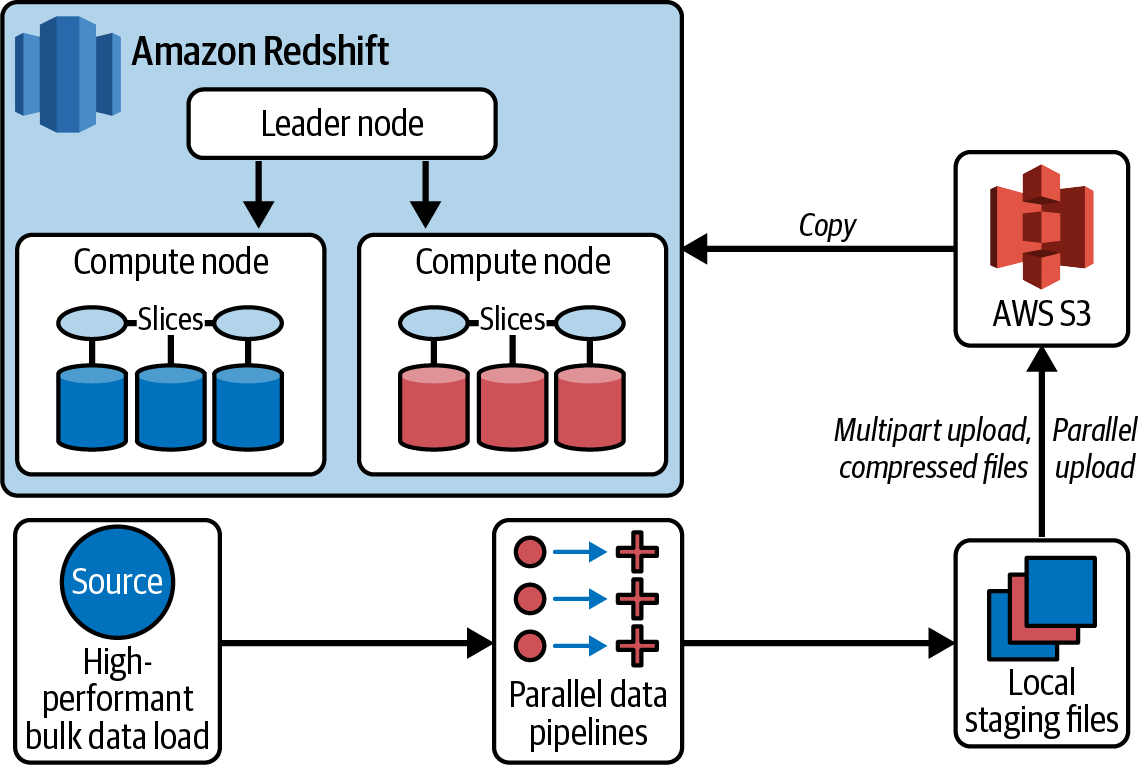
Figure 4-9. Informatica Amazon Redshift architecture

AWS Glue

AWS Glue is one of the native serverless data integration services commonly used to transform data using Python or Scala language and run on a data processing engine. With AWS Glue (Figure 4-10), you can read Amazon S3 data, apply transformations, and ingest data into Amazon Redshift data warehouses as well other data platforms. AWS Glue makes it easier to discover, prepare, move, and integrate data from multiple sources for analytics, ML, and application development. It offers multiple data integration engines, which include AWS Glue for Apache Spark, AWS Glue for Ray, and AWS Glue for Python Shell. You can use the appropriate engine for your workload, based on the characteristics of your workload and the preferences of your developers and analysts.

Figure 4-10. ETL integration using AWS Glue

Since AWS Glue V4, a new Amazon Redshift Spark connector with a new JDBC driver is featured with AWS Glue ETL jobs. You can use it to build Apache Spark applications that read from and write to data in Amazon Redshift as part of your data ingestion and transformation pipelines. The new connector and driver supports pushing down relational operations such as joins, aggregations, sort, and scalar functions from Spark to Amazon Redshift to improve your job performance by reducing the amount of data needing to be processed. It also supports IAM-based roles to enable single sign-on capabilities and integrates with AWS Secrets Manager for securely managing keys.

To manage your AWS Glue jobs, AWS provides a visual authoring tool, AWS Glue Studio. This service follows many of the same best practices as the third-party ETL tools already mentioned; however, because of the integration, it requires fewer steps to build and manage your data pipelines.

In Example 4-26, we will build a job that loads incremental transaction data from Amazon S3 and merge it into a lineitem table using the key (l_orderkey, l⁠_⁠l⁠i⁠n⁠e​n⁠u⁠m⁠b⁠e⁠r) in your Amazon Redshift data warehouse.

Example 4-26. Create lineitem table

CREATE TABLE IF NOT EXISTS lineitem (
  L_ORDERKEY varchar(20) NOT NULL,
  L_PARTKEY varchar(20),
  L_SUPPKEY varchar(20),
  L_LINENUMBER integer NOT NULL,
  L_QUANTITY varchar(20),
  L_EXTENDEDPRICE varchar(20),
  L_DISCOUNT varchar(20),
  L_TAX varchar(20),
  L_RETURNFLAG varchar(1),
  L_LINESTATUS varchar(1),
  L_SHIPDATE date,
  L_COMMITDATE date,
  L_RECEIPTDATE date,
  L_SHIPINSTRUCT varchar(25),
  L_SHIPMODE varchar(10),
  L_COMMENT varchar(44));

To build a Glue job, we will follow the instructions in the next two sections.

Register Amazon Redshift target connection

Navigate to “Create connection” to create a new AWS Glue connection. Name the connection and choose the connection type of Amazon Redshift (see Figure 4-11).

Figure 4-11. Amazon Redshift connection name

Next, select the database instance from the list of autodiscovered Amazon Redshift data warehouses found in your AWS account and region. Set the database name and access credentials. You have an option of either setting a username and password or using AWS Secrets Manager. Finally, click “Create connection” (see Figure 4-12).

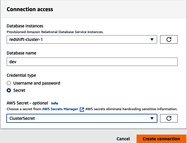
Figure 4-12. Amazon Redshift connection instance

Build and run your AWS Glue job

To build an AWS Glue job, navigate to the AWS Glue Studio jobs page. You will see a dialog prompting you with options for your job (Figure 4-13). In this example, we will select “Visual with a source and target.” Modify the target to Amazon Redshift and select Create.

Figure 4-13. AWS Glue Create job

Next, you will be presented with a visual representation of your job. The first step will be to select the data source node and set the S3 source type (Figure 4-14). For our use case we’ll use an S3 location and enter the location of our data: s3://redshift-immersionday-labs/data/lineitem-part/. Choose the parsing details such as the data format, delimiter, escape character, etc. For our use case, the files will have a CSV format, are pipe (|) delimited, and do not have column headers. Finally, click the “Infer schema” button.

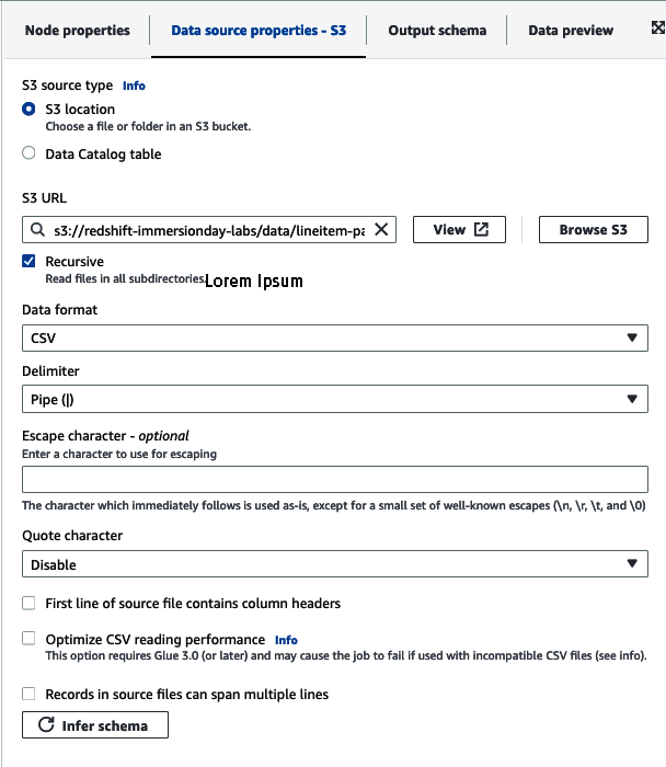
Figure 4-14. AWS Glue set Amazon S3 bucket

If you have established a data lake that you are using for querying with other AWS services like Amazon Athena, Amazon EMR, or even Amazon Redshift as an external table, you can alternatively use the “Data Catalog table” option.

Next, we can transform our data (Figure 4-15). The job is built with a simple ApplyMapping node, but you have many options for transforming your data such as joining, splitting, and aggregating data. See “Editing AWS Glue Managed Data Transform Nodes” AWS documentation for additional transform nodes. Select the Transform node and set the target key that matches the source key. In our case, the source data did not have column headers and were registered with generic columns (col#). Map them to the corresponding columns in your lineitem table.

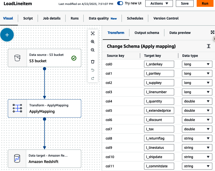
Figure 4-15. AWS Glue apply mapping

Now you can set the Amazon Redshift details (Figure 4-16). Choose “Direct data connection” and select the applicable schema (public) and table (lineitem). You can also set how the job will handle new records; you can either just insert every record or set a key so the job can update data that needs to be reprocessed. For our use case, we’ll choose MERGE and set the key l_orderkey and l_linenumber. By doing so, when the job runs, the data will first be loaded into a staging table, then a MERGE statement will be run based on any data that already exists in the target before the new data is loaded with an INSERT statement.

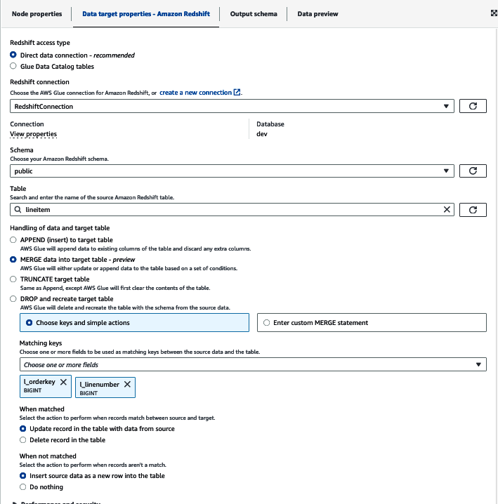
Figure 4-16. AWS Glue set Amazon Redshift target

Before you can save and run the job, you must set some additional job details like the IAM role, which will be used to run the job, and the script filename (Figure 4-17). The role should have permissions to access the files in your Amazon S3 location and should also be able to be assumed by the AWS Glue service. Once you have created and set the IAM role, click Save and Run to execute your job.

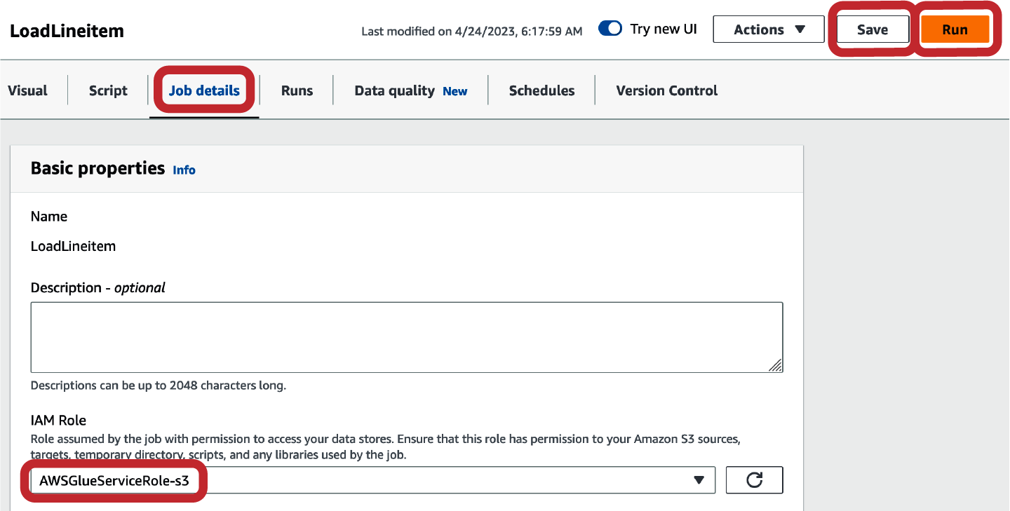
Figure 4-17. AWS Glue set job details

You can inspect the job run by navigating to the Runs tab. You will see details about the job ID and the run statistics (Figure 4-18).

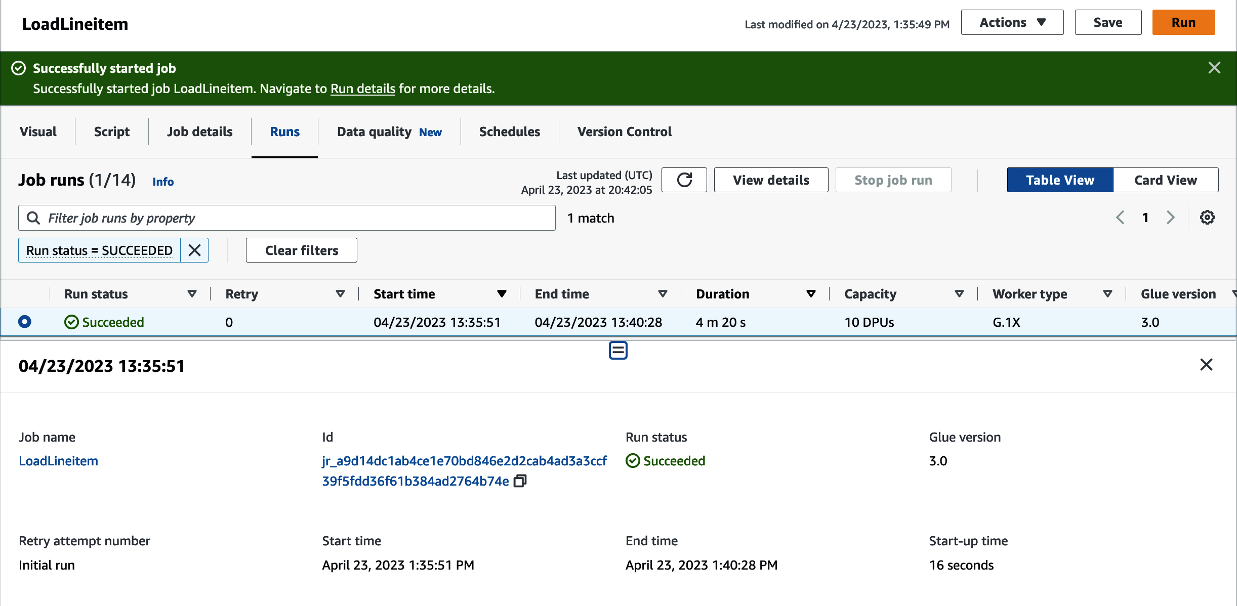
Figure 4-18. AWS Glue job run details

For AWS Glue to access Amazon S3, you will need to create a VPC endpoint if you have not created one already. See the online documentation for more details.

Once the job is completed, you can navigate to the Amazon Redshift console to inspect the queries and loads (Figure 4-19). You’ll see the queries required to create the temporary table, load the Amazon S3 files, and execute the merge statement that deletes old data and inserts new data.

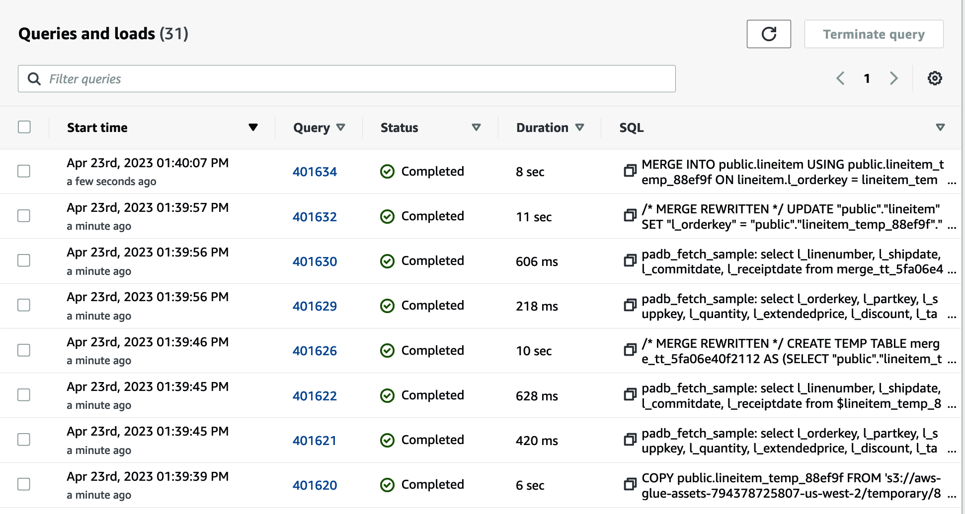
Figure 4-19. Amazon Redshift query history

Summary

This chapter described the various ways you can transform data using Amazon Redshift. With Amazon Redshift’s ability to access all your data whether it has been loaded or not, you can transform data in your data lake, operational sources, or other Amazon Redshift data warehouses quickly and easily. In addition, we showed that you can implement time-based schedules using the Amazon Redshift query scheduler to orchestrate these jobs. Lastly, we covered how Amazon Redshift partners with third-party ETL and orchestration vendors to provide optimal execution performance and integrate with tools you may already have in your organization.

In the next chapter, we’ll talk about how Amazon Redshift scales when you make changes to your workload. We’ll also cover how an Amazon Redshift serverless data warehouse will automatically scale and how you have control over how to scale your provisioned data warehouse. We’ll also talk about how you can get the best price performance with Amazon Redshift by implementing best practices.