Uncovering hidden patterns through machine learning
Lessons from FizzBuzz for Apache MXNet.
 Geometry (source: Pixabay)
When data scientist Joel Grus wrote an article on using machine learning to solve the “fizzbuzz” problem last year, most people saw it as an exercise in comedy, perhaps with a warning about the inappropriate use of AI. But we saw a deeper lesson. Certainly, you don’t need AI to solve fizzbuzz, so long as someone tells you the algorithm underlying the problem. But suppose you discover a seemingly random pattern like fizzbuzz output in nature? Patterns like that exist throughout real life, and no one gives us the algorithm. Machine learning solves such problems.
This summer, I had an opportunity to interview with an AI startup that I really liked. And guess what? I was asked to solve fizzbuzz using deep learning. Long story short, I didn’t get the job offer.
But this made us think about why fizzbuzz makes sense as an application of deep learning. On the surface, it’s a silly problem in integer arithmetic (or number theory, if you like to be pedantic). But it generates interesting patterns, and if you saw a list of inputs and outputs without knowing the underlying algorithm, finding a way to predict the outputs would be hard. Therefore, fizzbuzz is an easy way to generate patterns on which you can test deep learning techniques. In this article, we’ll try the popular Apache MXNet tools and find that this little exercise takes more effort than one might expect.
What is fizzbuzz ?
According to Wikipedia, fizzbuzz originated as children’s game, but for a long time has been a popular challenge that interviewers give programming candidates. Given an integer x, the programmer has to produce output according to the following rules:
- if
xis divisible by 3, output is “fizz” - if
xis divisible by 5, output is “buzz” - if
xis divisible by 15, output is “fizzbuzz” - else, the output is
x
A typical output sequence will look like this:
| Input | Output |
|---|---|
| 1 | 1 |
| 2 | 2 |
| 3 | “fizz” |
| 4 | 4 |
| 5 | “buzz” |
| 6 | “fizz” |
| 7 | 7 |
| 8 | 8 |
| 9 | “fizz” |
| 10 | “buzz” |
| 11 | 11 |
| 12 | “fizz” |
| 13 | 13 |
| 14 | 14 |
| 15 | “fizzbuzz” |
| 16 | 16 |
The requirements generate a surprisingly complex state machine, so they can reveal whether a novice programming candidate has good organizational skills. But if we know the rules that generate the data, there’s really no need for machine learning. Unfortunately, in real-life, we only have the data. Machine learning helps us create a model of the data. In this aspect, fizzbuzz provides us with an easy-to-understand data set and allows us to understand and explore the algorithms.
What follows is a pedantic exercise in understanding how MXNet can be used to solve the fizzbuzz problem.
What is MXNet?
MXNet is a scalable open source deep learning framework with a broad base of support. It is supported by Amazon, Intel, Dato, Baidu, Microsoft, and MIT among others.
MXNet offers the following advantages:
- Device Placement: It is easy to specify where each data structure should live (CPU versus GPU).
- Multi-GPU training: It is easy to scale the computations with more GPUs.
- Automatic differentiation: It automates the derivative calculations.
- Optimized Predefined Layers: The pre-defined layers are optimized for speed.
We use it in this article because of its popularity and because it is one of the most flexible frameworks in deep learning.
Structure of the article
In the subsequent sections, we will do the following:
- Structure the problem as a multi-class classification problem
- Generate the fizzbuzz data
- Divide the data into train and test
- Build a logistic regression model in MXNet from scratch
- Introduce
gluon - Build a multi-layer-perceptron model using
gluon
The examples are coded in Python because it is compact and well-known.
Structure the problem
Given the data, how do we structure this as a machine learning problem? To do supervised machine learning, we need features and a target variable. fizzbuzz can be modeled as a multi-class classification problem.
-
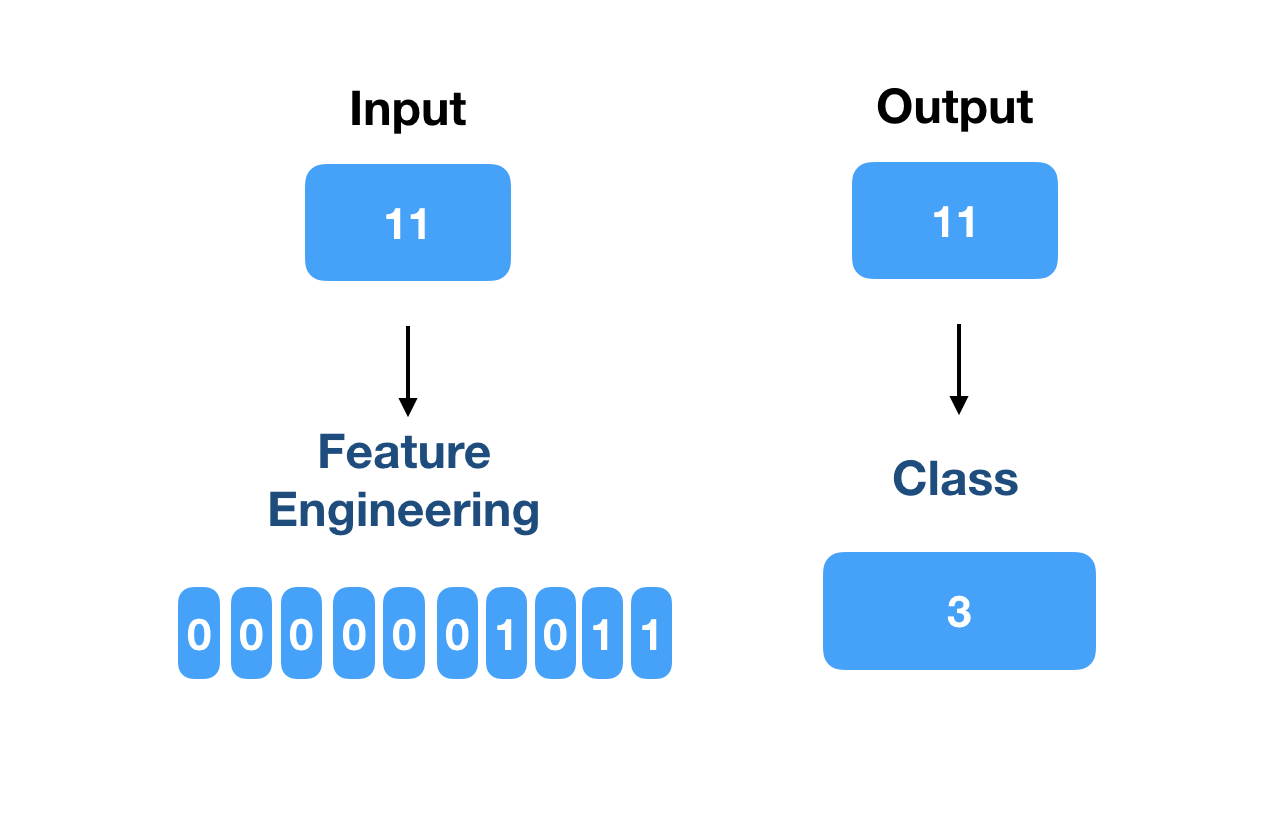
Input: Let’s think of a way to do feature engineering for the input. The input is an integer. One option, which Joel Grus employed in his article, is to convert the number to its binary representation. The binary representation can be fixed-length, and each digit of the fixed-length binary representation can be an input feature.
-
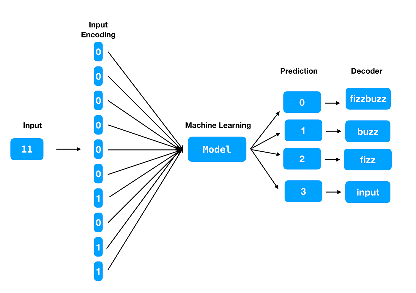
Target: The target can be one of the four classes—fizz, buzz, fizzbuzz, or the given number. The model should predict which of the classes is most likely for an input number. After the four classes are encoded and the model is built, it will return one of four prediction labels. So, we will also need a decoder function to convert the label to the corresponding output.
An example will explain this better.
Let’s say, we train the model using the first 1,000 integers. To create a binary representation of fixed length, we first need to find the maximum length of the input vector. All numbers up to 1,000 can be represented in binary within the size 210 (which is 1,024), so, we need the input vector to be of length 10.
The output is encoded in the prediction labels as 0, 1, 2, 3 for “fizzbuzz”, “buzz”, “fizz” and “the given number” respectively.
Example
Input: 11 (the given number)
Output: 11

Each digit of the input feature vector will be an input neuron. The output will have four neurons, one corresponding to each of the labels.
Figure 2 depicts this process.

Now let’s start building models using MXNet.
Installing and configuring MXNet
To get the software we need for this example, let’s first import the required Python libraries numpy and mxnet.
One way to install mxnet is to run the following command”
#install mxnet. If its already available, upgrade it.!pipinstallmxnet--upgrade--pre
#import librariesimportnumpyasnpimportmxnetasmximportosmx.random.seed(1)
In mxnet, every array has a context—either on a GPU or CPU.
The data size won’t be too high for this exercise, and a single CPU should suffice.
#Define the context to be CPUctx=mx.cpu()
Helper functions
We need a few helper functions to start with.
First, a function to convert the given input integer to its binary form.
#function to encode the integer to its binary representationdefbinary_encode(i,num_digits):returnnp.array([i>>d&1fordinrange(num_digits)])
Next, a function to encode the target into one of the four classes.
#function to encode the target into multi-classdeffizz_buzz_encode(i):ifi%15==0:return0elifi%5==0:return1elifi%3==0:return2else:return3
Once the model is built and we use it to predict the prediction label for a given number, we need a decoder function: a function that maps the prediction to the right output. The following function helps us do that:
#Given prediction, map it to the correct output labeldeffizz_buzz(i,prediction):ifprediction==0:return"fizzbuzz"elifprediction==1:return"buzz"elifprediction==2:return"fizz"else:returnstr(i)
Creating train, validation, test data sets
We now need to create the train, validation, and test data sets.
Let’s generate 100,000 data points, representing the integers from 1 to 100,000.
In ideal case, the train, validation, and test data sets are randomly selected. But for the sake of simplicity, let’s use the first 100 integers as test data set. (Because we know how fizzbuzz works, we know that the output values are distributed pretty evenly across all integers, so we don’t have to worry about where we sample test data. But remember that in a real-life setting, the input data set is shuffled and train, validation, and test data sets are chosen randomly.) Once we create the model, we will check the accuracy of the model by predicting on the test data set.
We will use the integers 101 to 50,000—essentially the bottom half of the data range—as the training data set. We will build the model using this data set.
We will use integers 50,001 to 100,000—the top half of the data range—as the validation data set. We could use this for hyper-parameter tuning, but in this exercise, we won’t be doing hyper-parameter tuning.
We start by defining the number of integers to generate:
#Number of integers to generateMAX_NUMBER=100000
This number also determines the length of the input feature vector. We determine the number of bits required for the binary representation, adding 1 because we round down the logarithm to the next lower integer.
#The input feature vector is determined by NUM_DIGITSNUM_DIGITS=np.log2(MAX_NUMBER).astype(np.int)+1
The train, test, and validation data sets are generated.
#Generate training dataset - both features and labelstrainX=np.array([binary_encode(i,NUM_DIGITS)foriinrange(101,np.int(MAX_NUMBER/2))])trainY=np.array([fizz_buzz_encode(i)foriinrange(101,np.int(MAX_NUMBER/2))])
#Generate validation dataset - both features and labelsvalX=np.array([binary_encode(i,NUM_DIGITS)foriinrange(np.int(MAX_NUMBER/2),MAX_NUMBER)])valY=np.array([fizz_buzz_encode(i)foriinrange(np.int(MAX_NUMBER/2),MAX_NUMBER)])
#Generate test dataset - both features and labelstestX=np.array([binary_encode(i,NUM_DIGITS)foriinrange(1,101)])testY=np.array([fizz_buzz_encode(i)foriinrange(1,101)])
Now that we’ve created the train, test, and validation data sets, let’s load them into instances of mxnet‘s iterator NDArrayIter. It allows us to specify batch size for training and to set a flag to shuffle the data or not.
#Define the parametersbatch_size=100num_inputs=NUM_DIGITSnum_outputs=4
#Create iterator for train, test and validation datasetstrain_data=mx.io.NDArrayIter(trainX,trainY,batch_size,shuffle=True)val_data=mx.io.NDArrayIter(valX,valY,batch_size,shuffle=True)test_data=mx.io.NDArrayIter(testX,testY,batch_size,shuffle=False)
We need to write another helper function to evaluate the accuracy of the model. After the predictions are generated, this function uses MXNet methods to return a floating-point number from 0 to 1 that indicates how well the function holds up against the validation data set.
#Function to evaluate accuracy of the modeldefevaluate_accuracy(data_iterator,net):acc=mx.metric.Accuracy()data_iterator.reset()fori,batchinenumerate(data_iterator):data=batch.data[0].as_in_context(ctx)label=batch.label[0].as_in_context(ctx)output=net(data)predictions=nd.argmax(output,axis=1)acc.update(preds=predictions,labels=label)returnpredictions,acc.get()[1]
Logistic regression from scratch
We have the data and the helper functions in place.
To understand a plain-vanilla neural network, let’s build a multi-class logistic regression model from scratch using MXNet. To build from scratch, this is what we need to do:
- Initialize weights and bias to random values
- Compute the forward pass
- For each observation, the input features and weights are multiplied, added with bias and passed onto the sigmoid function. That’s the predicted output for that input.
- Compute the error
- Update the weights and bias using gradient descent
- Repeat steps 2-4 until convergence or for a specific number of epochs
This article does a wonderful job of building a multi-class logistic regression from scratch using MXNet.
Also, mxnet comes with an autograd package, which enables automatic differentiation of NDArray operations and is used to compute the gradients of the loss function with respect to the model weights.
#import autograd packagefrommxnetimportautograd,nd
The first programming step is to initialize the bias and weight matrix.
#Initialize the weight and bias matrix#weights matrixW=nd.random_normal(shape=(num_inputs,num_outputs))#bias matrixb=nd.random_normal(shape=num_outputs)#Model parametersparams=[W,b]
The next step is to attach the autograd to calculate each parameter’s gradients.
forparaminparams:param.attach_grad()
We want the output to be the probability for each of the classes. The sum of the probabilities should sum to one, which we can get by running the following softmax function.
defsoftmax(y_linear):exp=nd.exp(y_linear-nd.max(y_linear))norms=nd.sum(exp,axis=0,exclude=True).reshape((-1,1))returnexp/norms
The loss function we will be using is softmax cross entropy. Cross-entropy maximizes the log-likelihood given to the correct labels. More about softmax cross-entropy can be read here.
#loss functiondefsoftmax_cross_entropy(yhat,y):return-nd.nansum(y*nd.log(yhat),axis=0,exclude=True)
We now define the model.
defnet(X):y_linear=nd.dot(X,W)+byhat=softmax(y_linear)returnyhat
For the model to learn (update) the model parameters (weights and biases), we need to define an optimizer. Stochastic gradient descent is one of the most popular methods to update the parameters.
#Define the optimizerdefSGD(params,lr):forparaminparams:param[:]=param-lr*param.grad
Lets execute the training loops. For each training step, batch_size determines the number of data points that will be passed through the network for it to learn. Once all data points are passed through the network, one epoch is completed. The parameter epochs define the number of times the entire data set has to be cycled through the training process. We’ll choose a fairly large number of epochs so we give the framework a good chance to learn the pattern.
#hyper parameters for the trainingepochs=100learning_rate=.01smoothing_constant=.01
Let’s now execute the training function.
foreinrange(epochs):#at the start of each epoch, the train data iterator is resettrain_data.reset()fori,batchinenumerate(train_data):data=batch.data[0].as_in_context(ctx)label=batch.label[0].as_in_context(ctx)label_one_hot=nd.one_hot(label,4)withautograd.record():output=net(data)loss=softmax_cross_entropy(output,label_one_hot)loss.backward()SGD(params,learning_rate)curr_loss=nd.mean(loss).asscalar()moving_loss=(curr_lossif((i==0)and(e==0))else(1-smoothing_constant)*moving_loss+(smoothing_constant)*curr_loss)#the training and validation accuracies are computed_,val_accuracy=evaluate_accuracy(val_data,net)_,train_accuracy=evaluate_accuracy(train_data,net)("Epoch%s. Loss:%s, Train_acc%s, Val_acc%s"%(e,moving_loss,train_accuracy,val_accuracy))
Epoch 99. Loss: 1.18811465231, Train_acc 0.532825651303, Val_acc 0.5332
For 100 epochs, the train accuracy and validation accuracy doesn’t seem great. It is only around 53%. Let’s check the accuracy on the test data set.
#model accuracy on the test datasetpredictions,test_accuracy=evaluate_accuracy(test_data,net)output=np.vectorize(fizz_buzz)(np.arange(1,101),predictions.asnumpy().astype(np.int))(output)("Test Accuracy : ",test_accuracy)
['1' '2' '3' '4' '5' '6' '7' '8' '9' '10' '11' '12' '13' '14' '15' '16'
'17' '18' '19' '20' '21' '22' '23' '24' '25' '26' '27' '28' '29' '30' '31'
'32' '33' '34' '35' '36' '37' '38' '39' '40' '41' '42' '43' '44' '45' '46'
'47' '48' '49' '50' '51' '52' '53' '54' '55' '56' '57' '58' '59' '60' '61'
'62' '63' '64' '65' '66' '67' '68' '69' '70' '71' '72' '73' '74' '75' '76'
'77' '78' '79' '80' '81' '82' '83' '84' '85' '86' '87' '88' '89' '90' '91'
'92' '93' '94' '95' '96' '97' '98' '99' '100']
Test Accuracy : 0.53
The accuracy on the test data set is also 53%. The model doesn’t seem to be working well.
What is gluon?
The gluon library in Apache MXNet provides a clear, concise, and simple API for deep learning. Gluon makes it easy to prototype, build, and train deep learning models without sacrificing training speed.
Gluon supports both imperative and symbolic programming, making it easy to train complex models imperatively. More details can be found here.
Multi-layer perceptron using gluon
Let’s build a multi-layer perceptron(MLP) model using gluon.
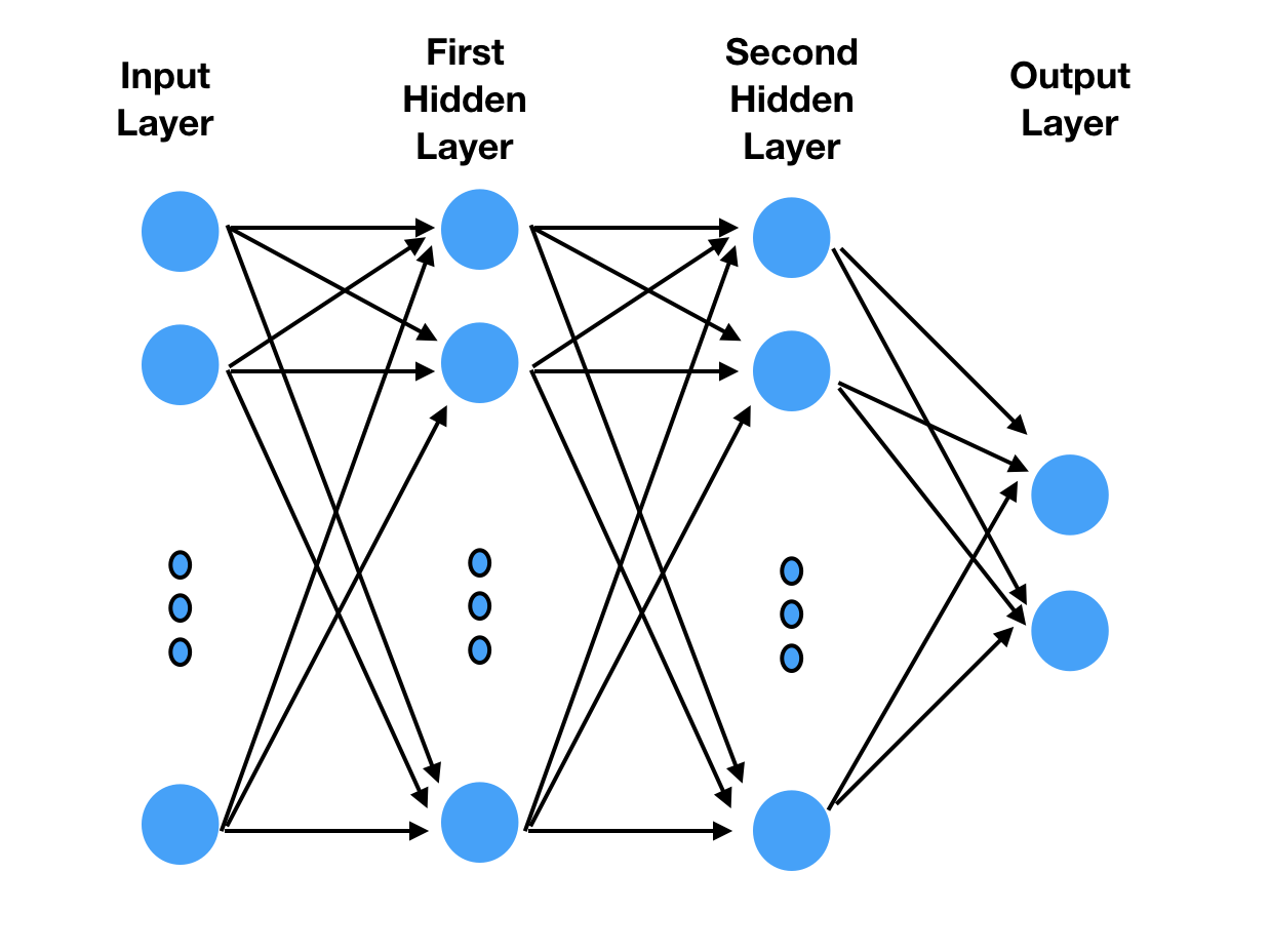
MLP is one of the simplest deep learning models. It runs data through multiple layers, using feedback to refine the processing layers (see Figure 3). More details can be found on Wikipedia.

We first need to import gluon:
#import gluonfrommxnetimportgluon
#reset the training, test and validation iteratorstrain_data.reset()val_data.reset()test_data.reset()
Now, define the gluon sequential model. Each hidden layer is added sequentially. The num_hidden variable defines the number of neurons in each of the hidden layers. The relu activation function is used in each of the layers.
#Define number of neurons in each hidden layernum_hidden=64#Define the sequential networknet=gluon.nn.Sequential()withnet.name_scope():net.add(gluon.nn.Dense(num_inputs,activation="relu"))net.add(gluon.nn.Dense(num_hidden,activation="relu"))net.add(gluon.nn.Dense(num_hidden,activation="relu"))net.add(gluon.nn.Dense(num_outputs))
Similar to the previous exercise, where we built the model from scratch, the parameters need to be initialized.
#initialize parametersnet.collect_params().initialize(mx.init.Xavier(magnitude=2.24),ctx=ctx)
The loss function is defined, as in the previous example, to be softmax cross entropy.
#define the loss functionloss=gluon.loss.SoftmaxCrossEntropyLoss()
The chosen optimizer is stochastic gradient descent, similar to the previous model. For this model, we define both the learning rate and momentum.
#Define the optimizertrainer=gluon.Trainer(net.collect_params(),'sgd',{'learning_rate':.02,'momentum':0.9})
As you can see, we changed some of the hyper-parameters: we used Xavier initializer, we added momentum to optimizer, we changed the learning rate, and we added multiple layers. The simplicity of changing these and experimenting with various architectures is one of the advantages of using gluon.
Let’s now train the MLP model.
#define variables/hyper-paramtersepochs=100moving_loss=0.best_accuracy=0.best_epoch=-1
#train the modelforeinrange(epochs):train_data.reset()fori,batchinenumerate(train_data):data=batch.data[0].as_in_context(ctx)label=batch.label[0].as_in_context(ctx)withautograd.record():output=net(data)cross_entropy=loss(output,label)cross_entropy.backward()trainer.step(data.shape[0])ifi==0:moving_loss=nd.mean(cross_entropy).asscalar()else:moving_loss=.99*moving_loss+.01*nd.mean(cross_entropy).asscalar()_,val_accuracy=evaluate_accuracy(val_data,net)_,train_accuracy=evaluate_accuracy(train_data,net)ifval_accuracy>best_accuracy:best_accuracy=val_accuracyifbest_epoch!=-1:('deleting previous checkpoint...')os.remove('mlp-%d.params'%(best_epoch))best_epoch=e('Best validation accuracy found. Checkpointing...')net.save_params('mlp-%d.params'%(e))("Epoch%s. Loss:%s, Train_acc%s, Val_acc%s"%(e,moving_loss,train_accuracy,val_accuracy))
Best validation accuracy found. Checkpointing...
Epoch 99. Loss: 0.021456909065, Train_acc 0.99498997996, Val_acc 0.44902
The training accuracy looks good, but validation accuracy is terrible. A possible cause is overfitting. In a practical setting, we would have shuffled the data and the train, validation, and test data sets would have had a better share of higher and lower bits.
Let’s now predict the model on the test data set.
#Load the parametersnet.load_params('mlp-%d.params'%(best_epoch),ctx)
#predict on the test datasetpredictions,test_accuracy=evaluate_accuracy(test_data,net)output=np.vectorize(fizz_buzz)(np.arange(1,101),predictions.asnumpy().astype(np.int))(output)("Test Accuracy : ",test_accuracy)
['1' '2' '3' '4' 'buzz' '6' '7' '8' 'fizz' 'buzz' '11' 'fizz' '13' '14'
'15' 'buzz' '17' 'fizz' '19' 'buzz' 'fizz' '22' '23' 'fizz' 'buzz' '26'
'fizz' '28' '29' 'fizzbuzz' '31' 'buzz' 'fizz' '34' 'buzz' 'fizz' '37'
'38' '39' 'buzz' '41' 'fizz' '43' 'buzz' '45' 'buzz' '47' 'fizz' '49'
'buzz' 'fizz' '52' '53' 'fizz' 'buzz' '56' 'fizz' '58' '59' 'fizz' 'buzz'
'62' 'fizz' '64' 'buzz' '66' '67' '68' '69' 'buzz' '71' 'fizz' '73' '74'
'75' '76' '77' '78' '79' 'buzz' 'fizz' '82' '83' 'fizz' 'buzz' '86' '87'
'88' '89' 'fizzbuzz' '91' '92' 'fizz' '94' 'buzz' 'fizz' '97' '98' '99'
'buzz']
Test Accuracy : 0.83
The test accuracy is 83%.
Adding more hidden layers led to an improvement of the accuracy. It is possible to experiment with more epochs and/or more hidden layers with different activation functions to see if accuracy improves.
Conclusion and next steps
This article gave a quick overview of how to get started with mxnet and gluon. With gluon, prototyping and experimenting with various architectures is much faster. And autograd allows us to record computation history on the fly so as to calculate gradients later.
And we’ve seen that fizzbuzz is more complex than it seems at first, and provides a nice basis for studying different machine learning approaches.
The straight dope has a good set of tutorials to get started with mxnet.
This post is part of a collaboration between O’Reilly and Amazon. See our statement of editorial independence.
