The Theory and Practice of Investment Management: Asset Allocation, Valuation, Portfolio Construction, and Strategies, Second Edition

BINOMIAL TREES

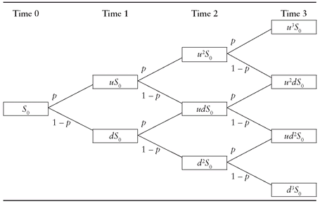
Binomial trees (also called binomial lattices) provide a natural way to model the dynamics of a random process over time. The initial value of the security S₀ (at time 0) is known. The length of a time period, Δt, is specified before the tree is built.⁷⁷ The binomial tree model assumes that at the next time period, only two values are possible for the price; that is, the price may go up with probability p or down with probability (1–p). Usually, these values are represented as multiples of the price at the beginning of the period. The factor u is used for an up movement, and d is used for a down movement. For example, the two prices at the end of the first time period are u ·S₀ and d · S₀. If the tree is recombining, there will be three possible prices at the end of the second time period: u² · S₀, u · d · S₀, and d² · S₀. Proceeding in a similar manner, we can build the tree in Exhibit 6.2.

EXHIBIT 6.2 Example of a Binomial Tree

The binomial tree model may appear simple because, given a current price, it only allows for two possibilities for the price at each time period. However, if the length of the time period is small, it is possible to represent a wide range of values for the price after only a few steps. To see this, notice that each step in the tree can be thought of as a Bernoulli trial⁷⁸—it is a “success” with probability p, and a “failure” with probability ...