Chapter 1. System Design Trade-offs and Guidelines
Today’s modern technological revolution is happening because of large scale software systems. Big enterprise companies like Google, Amazon, Oracle, and SAP have all built large scale software systems to run their (and their customer’s) businesses. Building and operating such large scale software systems requires first principles thinking to design and develop the technical architecture before actually putting the system into code. This is because we don’t want to be in a state where these systems will not work/scale after writing 10k lines of code. If the design is right in the first place, the rest of the implementation journey becomes smooth. This requires looking at the business requirements, understanding the needs and objectives of the customer, evaluating different trade-offs, thinking about error handling and edge cases, contemplating futuristic changes and robustness while worrying about basic details like algorithms and data structures. Enterprises can avoid the mistake of wasted software development effort by carefully thinking about systems and investing time in understanding bottlenecks, system requirements, users being targeted, user access patterns and many such decisions, which in short, is System Design.
This chapter covers the basics of system design, with the goal of helping you to understand the concepts around system design itself, the system trade-offs that naturally arise in such large-scale software systems, the fallacies to avoid in building such large scale systems and the guidelines—those wisdoms which were learnt after building such large scale software systems over the years. This is simply meant to introduce you to the basics—we’ll dig into details in later chapters, but we want you to have a good foundation to start with. Let’s begin by digging into the basic system design concepts.
System Design Concepts
To understand the building blocks of system design, we should understand the fundamental concepts around systems. We can leverage abstraction here, the concept in computer science of obfuscating the inner details to create a model of these system design concepts, which can help us to understand the bigger picture. The concepts in system design, be it any software system, revolve around communication, consistency, availability, reliability, scalability, fault tolerance and system maintainability. We will go over each of these concepts in detail, creating a mental model while also understanding how their nuances are applied in large scale system design.
Communication
A large scale software system is composed of small sub-systems, known as servers, which communicate with each other, i.e. exchange information or data over the network to solve a business problem, provide business logic, and compose functionality. Communication can take place in either a synchronous or asynchronous fashion, depending on the needs and requirements of the system.
Figure 1-1 shows the difference in the action sequence of both synchronous and asynchronous communication.
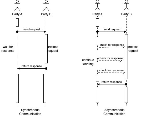
Figure 1-1. Sequence Diagram for Synchronous vs Asynchronous Communication
Let’s go over the details of both communication mechanisms in the following sections.
Note
We will cover the communication protocols as well as mechanisms for asynchronous communication in detail in Chapter 6: Communication Networks and Protocols.
Synchronous Communication
Consider a phone call conversation with your friend, you hear and speak with them at the same time and also use pauses in between to allow for conversation to complete. This is an example of synchronous communication, a type of communication in which two or more parties communicate with each other in real-time, with low latency. This type of communication is more immediate and allows for quicker resolution of issues or questions.
In system design, a communication mechanism is synchronous when the receiver will block (or wait) for the call or execution to return before continuing. This means that until a response is returned by the sender, the application will not execute any further, which could be perceived by the user as latency or performance lag in the application.
Asynchronous Communication
To give you an example of asynchronous communication, consider that instead of a phone call conversation, you switch to email. As you communicate over email with your friend, you send the message and wait for the reply at a later time (but within an acceptable time limit). You also follow a practice to follow up again if there is no response after this time limit has passed. This is an example of asynchronous communication, a type of communication in which two or more parties do not communicate with each other in real-time. Asynchronous communication can also take place through messaging platforms, forums, and social media, where users can post messages and responses may not be immediate.
In system design, a communication mechanism is asynchronous when the sender does not block (or wait) for the call or execution to return from the receiver. Execution continues on in your program or system, and when the call returns from the receiving server, a “callback” function is executed. In system design, asynchronous communication is often used when immediate response is not required, or when the system needs to be more flexible and tolerant of delays or failures.
In general, the choice of synchronous or asynchronous communication in system design depends on the specific requirements and constraints of the system. Synchronous communication is often preferred when real-time response is needed (such as the communication between the frontend UI and the backend), while asynchronous communication is often preferred when flexibility and robustness are more important (such as the communication to check the status of a long running job).
Consistency
Consistency, i.e. the requirement of being consistent, or in accordance with a set of rules or standards, is an important issue when it comes to communication between servers in a software system. Consistency can refer to a variety of concepts and contexts in system design.
In the context of distributed systems, consistency can be the property of all replica nodes (more on this in a moment) or servers having the same view of data at a given point in time. This means that all replica nodes have the same data, and any updates to the data are immediately reflected on all replica nodes.
In the context of data storage and retrieval, consistency refers to the property of each read request returning the value of the most recent write. This means that if a write operation updates the value of a piece of data, any subsequent read requests for that data should return the updated value. Let’s discuss each of these in more detail.
Consistency in Distributed Systems
Distributed systems are software systems, which are separated physically but connected over the network to achieve common goals using shared computing resources over the network.
Ensuring consistency, i.e. providing the same view of the data to each server in distributed systems can be challenging, as multiple replica servers may be located in different physical locations and may be subject to different failures or delays.
To address these challenges, we can use various techniques in distributed systems to ensure data consistency, such as:
- Data replication
-
In this approach, multiple copies of the data are maintained on different replica nodes, and updates to the data are made on all replica nodes simultaneously through blocking synchronous communication. This ensures that all replica nodes have the same view of the data at any given time.
- Consensus protocols
-
Consensus protocols are used to ensure that all replica nodes agree on the updates to be made to the data. They can use a variety of mechanisms, such as voting or leader election, to ensure that all replica nodes are in agreement before updating the data.
- Conflict resolution
-
In the event that two or more replica nodes try to update the same data simultaneously, conflict resolution algorithms are used to determine which update should be applied. These algorithms can use various strategies, such as last writer wins or merge algorithms, to resolve conflicts.
Overall, ensuring consistency in a distributed system is essential for maintaining the accuracy and integrity of the data, and various techniques are used to achieve this goal.
Consistency in Data Storage and Retrieval
Large scale software systems produce and consume a large amount of data and thus, ensuring consistency in such data storage and retrieval is important for maintaining the accuracy and integrity of the data in these systems. For example, consider a database that stores the balance of a bank account. If we withdraw money from the account, the database should reflect the updated balance immediately. If the database does not ensure consistency, it is possible for a read request to return an old balance, which could lead to incorrect financial decisions or even, financial loss for us or our banks.
To address these challenges, we can use various techniques in data storage systems to ensure read consistency, such as:
- Write-ahead logging
-
In this technique, writes to the data are first recorded in a log before they are applied to the actual data. This ensures that if the system crashes or fails, the data can be restored to a consistent state by replaying the log.
- Locking
-
Locking mechanisms are used to ensure that only one write operation can be performed at a time. This ensures that multiple writes do not interfere with each other and that reads always return the value of the most recent write.
- Data versioning
-
In this technique, each write operation is assigned a version number, and reads always return the value of the most recent version. This allows for multiple writes to be performed concurrently, while still ensuring that reads return the value of the most recent write.
Overall, ensuring consistency in data storage and retrieval is essential for maintaining the accuracy and integrity of the data, and various techniques are used to achieve this goal.
Note
We will discuss some of the above techniques for ensuring Consistency in detail in Chapter 2: Storage Types and Relational Stores and Chapter 3: Non-Relational Stores.
Consistency Spectrum Model
Since consistency can mean different things, the consistency spectrum model helps us reason about whether a distributed system is working correctly, when it’s doing multiple concurrent things at the same time like reading, writing, and updating data.
The consistency spectrum model represents the various consistency guarantees that a distributed system can offer, ranging from Eventual Consistency to Strong Consistency. The specific consistency guarantee chosen depends on the specific requirements and constraints of the system. Let’s walk through the consistency levels in the consistency spectrum model.
- Strong Consistency
-
At one end of the spectrum, strong consistency guarantees that all replica nodes have the same view of the data at all times, and that any updates to the data are immediately reflected on all replica nodes. This ensures that the data is always accurate and up-to-date, but can be difficult to achieve in practice, as it requires all replica nodes to be in constant communication with each other.
Note
We will cover the strong consistency requirements of relational databases as part of ACID property in Chapter 2: Storage Types and Relational Stores.
- Monotonic read consistency
-
Monotonic read consistency guarantees that once a client has read a value from a replica node, all subsequent reads from that client will return the same value or a more recent value. This means that a client will not see “stale” data that has been updated by another client. This provides a stronger consistency guarantee than eventual consistency, as it ensures that a client will not see outdated data.
- Monotonic write consistency
-
Monotonic write consistency guarantees that once a write operation has been acknowledged by a replica node, all subsequent reads from that replica node will return the updated value. This means that a replica node will not return outdated data to clients after a write operation has been acknowledged. This provides a stronger consistency guarantee than eventual consistency, as it ensures that a replica node will not return outdated data to clients.
- Causal consistency
-
Causal consistency works by categorizing operations into dependent and independent operations. Dependent operations are also called causally-related operations. Causal consistency preserves the order of the causally-related operations. It guarantees that if two operations are causally related into dependent and independant operations, then they will be seen in the same order by all processes in the system. This means that if operation A must happen before operation B, then all processes in the system will see A before they see B. This provides a stronger consistency guarantee than eventual consistency, as it ensures that the order of related operations is preserved.
- Eventual Consistency
-
At the other end of the spectrum, eventual consistency guarantees that, given enough time, all replica nodes will eventually have the same view of the data. This allows for more flexibility and tolerance of delays or failures, but can result in temporary inconsistencies in the data.
Note
We will cover the tunable consistency feature of some of the non-relational columnar databases like Cassandra in Chapter 3: Non-relational Stores.
Figure 1-2 shows the difference in the result of performing action sequence under strong consistency and eventual consistency. As you can see in the figure on the left for strong consistency, when x is read from a replica node after updating it from 0 to 2, it will block the request until replication happens and then, return 2 as result. On the other side in the figure on the right for eventual consistency, on querying the replica node, it will give stale result of x as 0 before replication completes.
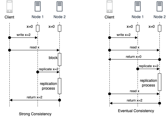
Figure 1-2. Sequence Diagram for Strong Consistency and Eventual Consistency
In general, the consistency spectrum model provides a framework for understanding the trade-offs between consistency and availability in distributed systems, and helps system designers choose the appropriate consistency guarantee for their specific needs.
Availability
In a large-scale software system, subsystems or servers can go down and may not be fully available to respond to the client’s requests — this is referred to as system’s availability. A system that is highly available is able to process requests and return responses in a timely manner, even under heavy load or in the face of failures or errors. Let’s try to quantify the measurement of availability of the system.
Measuring Availability
Availability can be measured mathematically as the percentage of the time the system was up (total time - time system was down) over the total time the system should have been running.
Availability percentages are represented in 9s, based on the above formula over a period of time. You can see the breakdown of what these numbers really work out to in Table 1-1.
| Availability % | Downtime per Year | Downtime per Month | Downtime per Week |
| 90% (1 nine) | 36.5 days | 72 hours | 16.8 hours |
| 99% (2 nines) | 3.65 days | 7.2 hours | 1.68 hours |
| 99.5% (2 nines) | 1.83 days | 3.60 hours | 50.4 minutes |
| 99.9% (3 nines) | 8.76 hours | 43.8 minutes | 10.1 minutes |
| 99.99% (4 nines) | 52.56 minutes | 4.32 minutes | 1.01 minutes |
| 99.999% (5 nines) | 5.26 minutes | 25.9 seconds | 6.05 seconds |
| 99.9999% (6 nines) | 31.5 seconds | 2.59 seconds | 0.605 seconds |
| 99.99999% (7 nines) | 3.15 seconds | 0.259 seconds | 0.0605 seconds |
The goal for availability is usually to achieve the highest level possible, such as “five nines” (99.999%) or even “six nines” (99.9999%). However, the level of availability that is considered realistic or achievable depends on several factors, including the complexity of the system, the resources available for maintenance and redundancy, and the specific requirements of the application or service.
Achieving higher levels of availability becomes progressively more challenging and resource-intensive. Each additional nine requires an exponential increase in redundancy, fault-tolerant architecture, and rigorous maintenance practices. It often involves implementing redundant components, backup systems, load balancing, failover mechanisms, and continuous monitoring to minimize downtime and ensure rapid recovery in case of failures.
While some critical systems, such as financial trading platforms or emergency services, may strive for the highest levels of availability, achieving and maintaining them can be extremely difficult and costly. In contrast, for less critical applications or services, a lower level of availability, such as 99% or 99.9%, may be more realistic and achievable within reasonable resource constraints.
Ultimately, the determination of what level of availability is realistic and achievable depends on a careful evaluation of the specific requirements, resources, costs, and trade-offs involved in each particular case.
Availability in parallel vs in sequence
The availability of a system that consists of multiple sub-systems depends on whether the components are arranged in sequence or in parallel with respect to serving the request.
Figure 1-3 shows the arrangement of components in sequential system on the left, where the request needs to be served from each component in sequence vs the parallel system on the right, where the request can be served from either component in parallel.
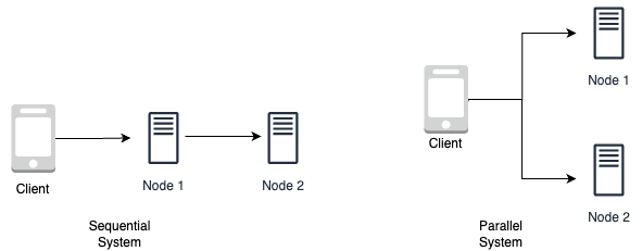
Figure 1-3. Sequential system vs Parallel system
If the components are in sequence, the overall availability of the service will be the product of the availability of each component. For example, if two components with 99.9% availability are in sequence, their total availability will be 99.8%.

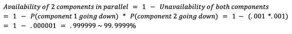
On the other hand, if the components are in parallel, the overall availability of the service will be the sum of the availability of each component minus the product of their unavailability. For example, if two components with 99.9% availability are in parallel, their total availability will be 99.9999%. This can lead to significantly higher availability compared to the same components arranged in sequence (6 9s from 3 9s in the above example).
Overall, the arrangement of components in a service can have a significant impact on its overall availability, and it is important to consider this when designing a system for high availability.
Ensuring Availability
Ensuring availability in a system is important for maintaining the performance and reliability of the system. There are several ways to increase the availability of a system, including:
- Redundancy
-
By having multiple copies of critical components or subsystems, a system can continue to function even if one component fails. This can be achieved through the use of redundant load balancers, failover systems, or replicated data stores.
- Fault tolerance
-
By designing systems to be resistant to failures or errors, the system can continue to function even in the face of unexpected events. This can be achieved through the use of error-handling mechanisms, redundant hardware, or self-healing systems.
- Load balancing
-
By distributing incoming requests among multiple servers or components, a system can more effectively handle heavy load and maintain high availability. This can be achieved through the use of multiple load balancers or distributed systems.
Note
We will cover load balancing in detail in Chapter 5: Scaling Approaches and Mechanisms and the different types of AWS load balancers in Chapter 9: AWS Network Services.
Overall, ensuring availability in a system is important for maintaining the performance and reliability of the system, and various techniques can be used to increase availability.
Availability Patterns
To ensure availability, there are two major complementary patterns to support high availability: fail-over and replication pattern.
Failover Patterns
Failover refers to the process of switching to a redundant or backup system in the event of a failure or error in the primary system. The failover pattern chosen depends on the specific requirements and constraints of the system, including the desired level of availability and the cost of implementing the failover solution. There are two main types of failover patterns: active-active and active-passive.
- Active-active failover
-
In an active-active failover pattern as shown on the left in Figure 1-4, multiple systems are used in parallel, and all systems are actively processing requests. If one system fails, the remaining systems can continue to process requests and maintain high availability. This approach allows for more flexibility and better utilization of resources, but can be more complex to implement and maintain.
- Active-passive failover
-
In an active-passive failover pattern as shown on the right in Figure 1-4, one system is designated as the primary system and actively processes requests, while one or more backup systems are maintained in a passive state. If the primary system fails, the backup system is activated to take over processing of requests. This approach is simpler to implement and maintain, but can result in reduced availability if the primary system fails, as there is a delay in switching to the backup system.
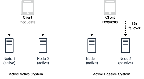
Figure 1-4. Active Active Failover system setup vs Active Passive Failover system setup
The failover pattern can involve the use of additional hardware and can add complexity to the system. There is also the potential for data loss if the active system fails before newly written data can be replicated to the passive system. Overall, the choice of failover pattern depends on the specific requirements and constraints of the system, including the desired level of availability and the cost of implementing the failover solution.
Note
These failover patterns are employed in relational datastores, non-relational data stores and caches, and load balancers, which we will cover in detail in Chapter 2: Storage Types and Relational Stores, Chapter 3: Non-relational Stores, Chapter 4: Caching Policies and Strategies and Chapter 5: Scaling Approaches and Mechanisms respectively.
Replication Patterns
Replication is the process of maintaining multiple copies of data or other resources in order to improve availability and fault tolerance. The replication pattern chosen depends on the specific requirements and constraints of the system, including the desired level of availability and the cost of implementing the replication solution.
There are two main types of replication patterns: Multi leader and Single leader.
- Multi leader replication
-
In a multi leader replication pattern as shown on the left in Figure 1-5, multiple systems are used in parallel and all systems are able to both read and write data. This allows for more flexibility and better utilization of resources, as all systems can process requests and updates to the data simultaneously. A load balancer is required or application logic changes need to be made to support multiple leaders and identify on which leader node to write. Most multi leader systems are either loosely consistent or have increased write latency due to synchronization to remain consistent. Conflict resolution comes more into play as more write nodes are added, leading to increase in latency. However, this approach can become more complex to implement and maintain, as it requires careful management of conflicts and errors.
- Single leader replication
-
In a single leader replication pattern as shown on the right in Figure 1-5, one system is designated as the leader system and is responsible for both reading and writing data, while one or more follower systems are used to replicate the data. The follower systems can only be used for reading data, and updates to the data must be made on the leader system. Additional logic is required to be implemented to promote a follower to the leader. This approach is simpler to implement and maintain, but can result in reduced availability if the leader system fails, as updates to the data can only be made on the leader system and there is a risk of losing the data updates.
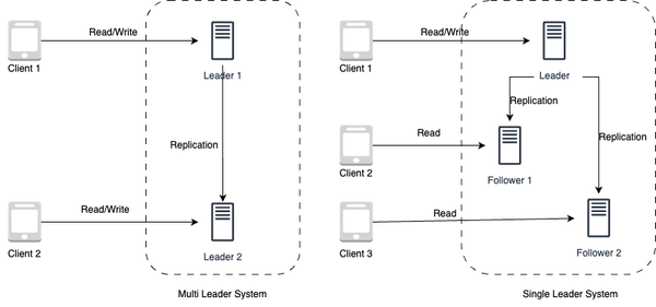
Figure 1-5. Multi-leader replication system setup vs Single leader replication system setup
There is a risk of data loss if the leader system fails before newly written data can be replicated to other nodes. And thus, the more read replicas that are used, the more writes need to be replicated, which can lead to greater replication lag. In addition, the use of read replicas can impact the performance of the system, as they may be bogged down with replaying writes and unable to process as many reads. Furthermore, replication can involve the use of additional hardware and can add complexity to the system. Finally, some systems may have more efficient write performance on the leader system, as it can spawn multiple threads to write in parallel, while read replicas may only support writing sequentially with a single thread. Overall, the choice of replication pattern depends on the specific requirements and constraints of the system, including the desired level of availability and the cost of implementing the replication solution.
Note
We will cover how relational and non-relational datastores ensure availability using single leader and multi-leader replication in Chapter 2: Storage Types and Relational Stores and Chapter 3: Non-relational Stores. Do look out for leaderless replication using consistent hashing to ensure availability in non-relational stores like key-value stores and columnar stores in detail in Chapter 3: Non-relational Stores.
Reliability
In system design, reliability refers to the ability of a system or component to perform its intended function consistently and without failure over a given period of time. It is a measure of the dependability or trustworthiness of the system. Reliability is typically expressed as a probability or percentage of time that the system will operate without failure. For example, a system with a
reliability of 99% will fail only 1% of the time. Let’s try to quantify the measurement of reliability of the system.
Measuring Reliability
One way to measure the reliability of a system is through the use of mean time between failures(MTBF) and mean time to repair (MTTR).
- Mean time between failures
-
Mean time between failures (MTBF) is a measure of the average amount of time that a system can operate without experiencing a failure. It is typically expressed in hours or other units of time. The higher the MTBF, the more reliable the system is considered to be.
- Mean time to repair
-
Mean time to repair (MTTR) is a measure of the average amount of time it takes to repair a failure in the system. It is also typically expressed in hours or other units of time. The lower the MTTR, the more quickly the system can be restored to operation after a failure.
Together, MTBF and MTTR can be used to understand the overall reliability of a system. For example, a system with a high MTBF and a low MTTR is considered to be more reliable than a system with a low MTBF and a high MTTR, as it is less likely to experience failures and can be restored to operation more quickly when failures do occur.
Reliability and Availability
It is important to note that reliability and availability are not mutually exclusive. A system can be both reliable and available, or it can be neither. A system that is reliable but not available is not particularly useful, as it may be reliable but not able to perform its intended function when needed.
On the other hand, a system that is available but not reliable is also not useful, as it may be able to perform its intended function when needed, but it may not do so consistently or without failure. In order to achieve high reliability and availability to meet agreed service level objectives (SLO), it is important to design and maintain systems with redundant components and robust failover mechanisms. It is also important to regularly perform maintenance and testing to ensure that the system is operating at its optimal level of performance.
In general, the reliability of a system is an important consideration in system design, as it can impact the performance and availability of the system over time.
Note
Service level objectives and goals including Change Management, Problem Management and Service Request Management of AWS Managed Services, which will be introduced in section 2 - Diving Deep into AWS Services are provided in AWS documentation here.
Scalability
In system design, we need to ensure that the performance of the system increases with the resources added based on the increasing workload, which can either be request workload or data storage workload. This is referred to as scalability in system design, which requires the system to respond to increased demand and load. For example, a social network needs to scale with the increasing number of users as well as the content feed on the platform, which it indexes and serves.
Scalability Patterns
To ensure scalability, there are two major complementary patterns to scale the system: vertical scaling and horizontal scaling.
Vertical Scaling
Vertical scaling involves meeting the load requirements of the system by increasing the capacity of a single server by upgrading it with more resources (CPU, RAM, GPU, storage etc) as shown on the left in Figure 1-6. Vertical scaling is useful when dealing with predictable traffic, as it allows for more resources to be used to handle the existing demand. However, there are limitations to how much a single server can scale up based on its current configuration and also, the cost of scaling up is generally high as adding more higher end resources to the existing server will require more dollars for high end configurations.
Horizontal Scaling
Horizontal scaling involves meeting the load requirements of the system by increasing the number of the servers by adding more commodity servers to serve the requests as shown on the right in Figure 1-6. Horizontal scaling is useful when dealing with unpredictable traffic, as adding more servers increases the servers capacity to handle more requests and if demand arises, more servers can further be added to the pool cost-effectively However, though horizontal scaling provides a better dollar cost proposition for scaling, the complexity of managing multiple servers and ensuring they work collectively as an abstracted single server to handle the workload is the catch here.
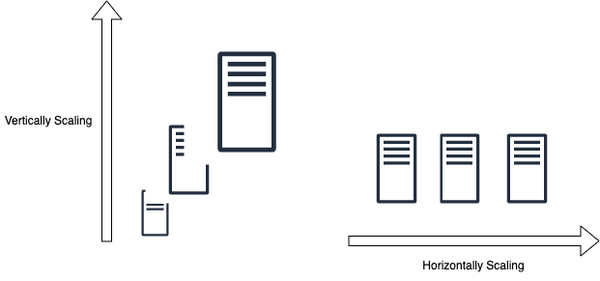
Figure 1-6. Vertical Scaling vs Horizontal Scaling
Note
We will cover both scaling approaches and mechanisms in detail in Chapter 5: Scaling Approaches and Mechanisms.
In early stage systems, you can start scaling up by vertically scaling the system and adding better configuration to it and later, when you hit the limitation in further scaling up, you can move to horizontally scaling the system.
Maintainability
In system design, maintainability is the ability of the system to be modified, adapted, or extended to meet the changing needs of its users while ensuring smooth system operations. In order for a software system to be maintainable, it must be designed to be flexible and easy to modify or extend.
The maintainability of a system requires covering these three underlyings aspects of the system:
- Operability
-
This requires the system to operate smoothly under normal conditions and even return back to normal operations within stipulated time after a fault. When a system is maintainable in terms of operability, it reduces the time and effort required to keep the system running smoothly. This is important because efficient operations and management contribute to overall system stability, reliability, and availability.
- Lucidity
-
This requires the system to be simple and lucid to understand, extend to add features and even, fix bugs. When a system is lucid, it enables efficient collaboration among team members, simplifies debugging and maintenance tasks, and facilitates knowledge transfer. It also reduces the risk of introducing errors during modifications or updates.
- Modifiability
-
This requires the system to be built in a modular way to allow it to be modified and extended easily, without disrupting the functionality of other subsystems. Modifiability is vital because software systems need to evolve over time to adapt to new business needs, technological advancements, or user feedback. A system that lacks modifiability can become stagnant, resistant to change, and difficult to enhance or adapt to future demands.
By prioritizing maintainability, organizations can reduce downtime, lower maintenance costs, enhance productivity, and increase the longevity and value of their software systems.
Fault Tolerance
Large scale systems generally employ a large number of servers and storage devices to handle and respond to the user requests and store data. Fault tolerance requires the system to recover from any failure (either hardware or software failure) and continue to serve the requests. This requires avoiding single points of failure in the large system and the ability to reroute requests to the functioning sub-systems to complete the workload.
Fault tolerance needs to be supported at hardware as well as software levels, while ensuring the data safety, i.e. making sure we don’t lose the data. There are two major mechanisms to ensure data safety: replication and checkpointing.
Replication
Replication based fault tolerance ensures data safety as well as serving the request by replicating both the service through multiple replica servers and also, replicating the data through multiple copies of data across multiple storage servers. During a failure, the failed node gets swapped with a fully functioning replica node. Similarly data is also served again from a replica store, in case the data store has failed. The replication patterns were already covered in the previous section in availability.
Checkpointing
Checkpointing based fault tolerance ensures that data is reliably stored and backed up, even after the initial processing is completed. It allows for a system to recover from any potential data loss, as it can restore a previous system state and prevent data loss. Checkpointing is commonly used to ensure system and data integrity, especially when dealing with large datasets. It can also be used to verify that data is not corrupted or missing, as it can quickly detect any changes or issues in the data and then take corrective measures. Checkpointing is an important tool for data integrity, reliability, and security, as it ensures that all data is stored properly and securely.
Note
Recovery Manager of databases use checkpointing to ensure the durability and reliability of the database in the event of failures or crashes. This will be covered in detail in Chapter 2: Storage Types and Relational Stores.
There are two checkpointing patterns — it can be done in either using synchronous or asynchronous mechanisms.
- Synchronous checkpointing
-
Synchronous checkpointing in a system is achieved by stopping all the data mutation requests and allowing only read requests, while waiting for all the checkpointing process to complete for the current data mutation to ensure its integrity across all nodes. This always ensures consistent data state across all the nodes.
- Asynchronous checkpointing
-
Asynchronous checkpointing in a system is done by checkpointing asynchronously on all the nodes, while continuing to serve all the requests (including data mutation requests) without waiting for the acknowledgement of the checkpointing process to complete. This mechanism suffers from the possibility of having inconsistent data state across the servers.
So now we have covered the basic concepts and requirements of a large scale system and strive towards building a performant and scalable system—one that is also highly available, reliable, maintainable and is fault-tolerant. Before diving deep into how to build such systems, let’s go through the inherent fallacies as well as trade-offs in designing such systems.
Fallacies of Distributed Computing
As a large-scale software system involves multiple distributed systems, it is often subject to certain fallacies that can lead to incorrect assumptions and incorrect implementations. These fallacies were first introduced by L. Peter Deutsch and they cover the common false assumptions that software developers make while implementing distributed systems. These eight fallacies are:
- Reliable Network
-
The first fallacy is assuming that “The network is reliable”. Networks are complex, dynamic and often, unpredictable. Small issues like switch or power failures can even bring the entire network of a data-center down, making the network unreliable. Thus, it is important to account for the potential of an unreliable network while designing large scale systems, ensuring network fault tolerance from the start. Given that networks are inherently unreliable, to build reliable services on top we must rely on protocols that can cope with network outages and packet loss.
- Zero Latency
-
The second fallacy is assuming that “Latency is zero”. Latency is an inherent limitation of networks, constrained by the speed of light, i.e. even in perfect theoretical systems, the data can’t reach faster than the speed of light between the nodes. Hence, to account for latency, the system should be designed to bring the clients close to data through edge-computing and even choosing the servers in the right geographic data centers closer to the clients and routing the traffic wisely.
- Infinite Bandwidth
-
The third fallacy is assuming that “Bandwidth is infinite”. When a high volume of data is flowing through the network, there is always network resource contention leading to queueing delays, bottlenecks, packet drops and network congestion. Hence, to account for finite bandwidth, build the system using lightweight data formats for the data in transit to preserve the network bandwidth and avoid network congestion. Or use multiplexing, a technique that improves bandwidth utilization by combining data from several sources and send it over the same communication channel/medium.
- Secure Network
-
The fourth fallacy is assuming that “The network is secure”. Assuming a network is always secure, when there are multiple ways a network can be compromised (ranging from software bugs, OS vulnerabilities, viruses and malwares, cross-site scripting, unencrypted communication, malicious middle actors etc) can lead to system compromise and failure. Hence to account for insecure networks, build systems with a security first mindset and perform defense testing and threat modelling of the built system.
- Fixed Topology
-
The fifth fallacy is assuming that “Topology doesn’t change”. In distributed systems, the topology changes continuously, because of node failures or node additions. Building a system that assumes fixed topology will lead to system issues and failures due to latency and bandwidth constraints. Hence, the underlying topology must be abstracted out and the system must be built oblivious to the underlying topology and tolerant to its changes.
- Single Administrator
-
The sixth fallacy is assuming that “There is one administrator”. This can be a fair assumption in a very small system like a personal project, but this assumption breaks down in large scale distributed computing, where multiple systems have separate OS, separate teams working on it and hence, multiple administrators. To account for this, the system should be built in a decoupled manner, ensuring repair and troubleshooting becomes easy and distributed too.
- Zero Transport cost
-
The seventh fallacy is assuming that “Transport cost is zero”. Network infrastructure has costs, including the cost of network servers, switches, routers, other hardwares, the operating software of these hardware, and the team cost to keep it running smoothly. Thus, the assumption that transporting data from one node to another is negligible is false and must consequently be noted in budgets to avoid vast shortfalls.
- Homogenous Network
-
The eight fallacy is assuming that “The network is homogeneous”. A network is built with multiple devices with different configurations and using multiple protocols at different layers and therefore we can’t assume a network is homogenous. Taking into consideration the heterogeneity of the network as well as focusing on the interoperability of the system,( i.e. ensuring subsystems can communicate and work together despite having such differences) will help to avoid this pitfall.
Note
The AWS Well-Architected Framework consists of six core pillars that provide guidance and best practices for designing and building systems on the AWS cloud, avoiding these fallacies and pitfalls.
Operational Excellence pillar avoids the fallacy of Single Administrator and Homogenous Network. Security pillar avoids the fallacy of Secure Network. Reliability pillar avoids the fallacy of Reliable Network and Fixed Topology. Performance Efficiency pillar avoids the fallacy of Zero Latency and Infinite Bandwidth. Cost Optimization pillar as well as Sustainability pillar avoids the fallacy of Zero Transport Cost.
The book will not cover the AWS Well-Architected Framework in detail and it is left as an excursion for the readers.
These fallacies cover the basic assumptions we should avoid while building large scale systems. Overall, neglecting the fallacies of distributed computing can lead to a range of issues, including system failures, performance bottlenecks, data inconsistencies, security vulnerabilities, scalability challenges, and increased system administration complexity. It is important to acknowledge and account for these fallacies during the design and implementation of distributed systems to ensure their robustness, reliability, and effective operation in real-world environments. Lets also, go through the trade-offs in the next section, which are generally encountered in designing large scale software systems.
System Design Trade-offs
System design involves making a number of trade-offs that can have a significant impact on the performance and usability of a system. When designing a system, you must consider factors like cost, scalability, reliability, maintainability, and robustness. These factors must be balanced to create a system that is optimized for the particular needs of the user. Ultimately, the goal is to create a system that meets the needs of the user without sacrificing any of these important factors.
For example, if a system needs to be highly reliable but also have scalability, then you need to consider the trade-offs between cost and robustness. A system with a high level of reliability may require more expensive components, but these components may also be robust and allow for scalability in the future. On the other hand, if cost is a priority, then you may have to sacrifice robustness or scalability in order to keep the system within budget.
In addition to cost and scalability, other trade-offs must be taken into account when designing a system. Performance, security, maintainability, and usability are all important considerations that must be weighed when designing a system. There are some theoretical tradeoffs that arise in system design, which we will discuss in this section.
Time vs Space
Space time trade-offs or time memory trade-offs arise inherently in implementation of the algorithms in computer science for the workload, even in distributed systems. This trade-off is necessary because system designers need to consider the time limitations of the algorithms and sometimes use extra memory or storage to make sure everything works optimally. One example of such a trade-off is in using look-up tables in memory or data storage instead of performing recalculation and thus, serving more requests by just looking up pre-calculated values.
Latency vs Throughput
Another trade-off that arises inherently in system design is latency vs throughput. Before diving into the trade-off, let’s make sure you understand these concepts thoroughly.
- Latency, Processing time and Response time
-
Latency is the time that a request waits to be handled. Until the request is picked up to be handled, it is latent, inactive, queued or dormant.
-
Processing time, on the other hand, is the time taken by the system to process the request, once it is picked up.
-
Hence, the overall response time is the duration between the request that was sent and the corresponding response that was received, accounting for network and server latencies.
-
Mathematically, it can be represented by the following formula:
- Throughput and Bandwidth
-
Throughput and bandwidth are metrics of network data capacity, and are used to account for network scalability and load. Bandwidth refers to the maximum amount of data that could, theoretically, travel from one point in the network to another in a given time. Throughput refers to the actual amount of data transmitted and processed throughout the network. Thus, bandwidth describes the theoretical limit, throughput provides the empirical metric. The throughput is always lower than the bandwidth unless the network is operating at its maximum efficiency.
Bandwidth is a limited resource as each network device can only handle and process limited capacity of data before passing it to the next network device, and some devices consume more bandwidth than others. Insufficient bandwidth can lead to network congestion, which slows connectivity.
Since latency measures how long the packets take to reach the destination in a network while throughput measures how many packets are processed within a specified period of time, they have an inverse relationship. The more the latency the more they would get queued up in the network, reducing the number of packets that are being processed, leading to lower throughput.
Since the system is being gauged for lower latency under high throughput or load, the metric to capture latency is through percentiles like p50, p90, p99 and so on. For example, the p90 latency is the highest latency value (slowest response) of the fastest 90 percent of requests. In other words, 90 percent of requests have responses that are equal to or faster than the p90 latency value. Note that average latency of a workload is not used as a metric, as averages as point estimates are susceptible to outliers. Because of the latency vs throughput trade-off, the latency metric will go down as the load is increased on the system for higher throughput. Hence, systems should be designed with an aim for maximal throughput within acceptable latency.
Performance vs Scalability
As discussed earlier in the chapter, scalability is the ability of the system to respond to increased demand and load. On the other hand, performance is how fast the system responds to a single request. A service is scalable if it results in increased performance in a manner proportional to resources added. When a system has performance problems, it is slow for a single user (p50 latency = 100ms) while when the system has scalability problems, the system may be fast for some users (p50 latency = 1ms for 100 requests) but slow under heavy load for the users (p50 latency = 100ms under 100k requests).
Consistency vs Availability
As discussed earlier in the chapter, strong consistency in data storage and retrieval is the guarantee that every read receives the most recent write, while high availability is the requirement of the system to always provide a non-error response to the request. In a distributed system where the network fails (i.e. packets get dropped or delayed due to the fallacies of distributed computing leading to partitions) there emerges an inherent trade-off between strong consistency and high availability. This trade-off is called the CAP theorem, also known as Brewer’s theorem.
CAP Theorem
The CAP theorem, as shown in Venn Diagram Figure 1-7, states that it is impossible for a distributed system to simultaneously provide all three of the following guarantees: consistency (C), availability (A), and partition tolerance (P). According to the theorem, a distributed system can provide at most two of these guarantees at any given time. Systems need to be designed to handle network partitions as networks aren’t reliable and hence, partition tolerance needs to be built in. So, in particular, the CAP theorem implies that in the presence of a network partition, one has to choose between consistency and availability.
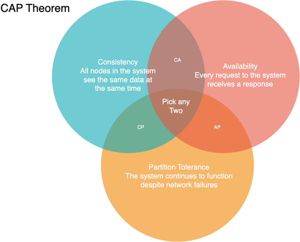
Figure 1-7. CAP Theorem Venn Diagram
However, CAP is frequently misunderstood as if one has to choose to abandon one of the three guarantees at all times. In fact, the choice is really between consistency and availability only when a network partition or failure happens; at all other times, the trade-off has to be made based on the PACLEC theorem.
PACELC Theorem
The PACELC theorem, as shown in Decision Flowchart Figure 1-8, is more nuanced version of CAP theorem, which states that in the case of network partitioning (P) in a distributed computer system, one has to choose between availability (A) and consistency (C) (as per the CAP theorem), but else (E), even when the system is running normally in the absence of partitions, one has to choose between latency (L) and consistency (C). This trade-off arises naturally because to handle network partitions, data and services are replicated in large scale systems, leading to the choice between the consistency spectrum and the corresponding latency.
If the system tries to provide for strong consistency at the one end of the consistency spectrum model, it has to do replication with synchronous communication and blocking to ensure all the read replicas receive the most recent write, waiting on the acknowledgement from all the replica nodes, adding to high latency. On the other hand, if the system does asynchronous replication without waiting for acknowledgment from all nodes, it will end up providing eventual consistency (i.e. the read request will eventually reflect the last recent write) when the replica node has acknowledged the data mutation change for serving the requests.
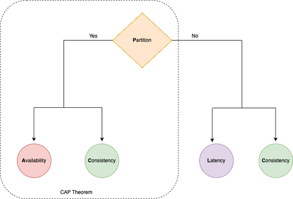
Figure 1-8. PACLEC Theorem Decision Flowchart
In summary, the CAP and PACELC theorems are important concepts in distributed systems design that provide a framework for understanding the trade-offs involved in designing highly available and strongly consistent systems.
Note
We will cover how non-relational stores navigate CAP theorem trade-off by providing BASE property in detail in Chapter 3: Non-relational Stores.
Given such requirements, fallacies and trade-offs in system design, in order to avoid repeating mistakes of the past we should prescribe to a set of guidelines learnt by the previous generation of software design practitioners. Let’s dig into those now.
System Design Guidelines
System design will always present the most interesting and challenging trade-offs, and a system designer should be aware of the hidden costs and be well-equipped to get it right — though not perfect! These guidelines, which have emerged over years of practicing system design, guide us to avoid pitfalls and handle trade-offs while designing large scale-systems. These guidelines aren’t just vague generalities but virtues that help reflect on why the system was designed the way it was, why it was implemented the way it is and why that was the right thing to do.
Guideline of Isolation: Build It Modularly
Controlling complexity is the essence of computer programming.
Brian Kernighan
The first guideline is to build the system modularly, i.e. break down a complex system into smaller, independent components or modules that can function independently, yet also work together to form the larger system. Building it modularly helps in improving all the requirements of the large scale system:
- Maintainability
-
Modules can be updated or replaced individually without affecting the rest of the system.
- Reusability
-
Modules can be reused in different systems or projects, reducing the amount of new development required.
- Scalability
-
Modules can be added or removed and even scaled independently as needed to accommodate changes in requirements or to support growth.
- Reliability
-
Modules can be tested and validated independently, reducing the risk of system-wide failures.
Modular systems can be implemented in a variety of ways, including through the use of microservices architecture, component-based development, and modular programming, which we will cover in more detail in chapter 7. However, designing modular systems can be challenging, as it requires careful consideration of the interfaces between modules, data sharing and flow, and dependencies.
Guideline of Simplicity: Keep it Simple, Silly
Everything should be made as simple as possible, but no simpler
Eric S. Raymond
The second guideline is to keep the design simple by avoiding complex and unnecessary features and avoiding over-engineering. To build simple systems using the KISS (Keep it Simple, Silly) guideline, designers can follow these steps:
-
1. Identify the core requirements: Determine the essential features and functions the system must have, and prioritize them.
-
2. Minimize the number of components: Reduce the number of components or modules in the system, making sure each component serves a specific purpose.
-
3. Avoid over-engineering: Don’t add unnecessary complexity to the system, such as adding features that are not necessary for its functioning.
-
4. Make the system easy to use: Ensure the system is intuitive and straightforward for users to use and understand.
-
5. Test and refine: Test the system to ensure it works as intended and make changes to simplify the system if necessary.
By following the KISS guideline, you as a system designer can build simple, efficient, and effective systems that are easy to maintain and less prone to failure.
Guideline of Performance: Metrics Don’t Lie
Performance problems cannot be solved only through the use of Zen meditation.
Jeffrey C. Mogul
The third guideline is to measure then build, and rely on the metrics as you can’t cheat the performance and scalability. Metrics and observability are crucial for the operation and management of large scale systems. These concepts are important for understanding the behavior and performance of large-scale systems and for identifying potential issues before they become problems.
- Metrics
-
Metrics are quantitative measures that are used to assess the performance of a system. They provide a way to track key performance indicators, such as resource utilization, response times, and error rates, and to identify trends and patterns in system behavior. By monitoring metrics, engineers can detect performance bottlenecks and anomalies, and take corrective actions to improve the overall performance and reliability of the system.
- Observability
-
Observability refers to the degree to which the state of a system can be inferred from its externally visible outputs. This includes being able to monitor system health and diagnose problems in real-time. Observability is important in large scale systems because it provides a way to monitor the behavior of complex systems and detect issues that may be impacting their performance.
Together, metrics and observability provide the information needed to make informed decisions about the operation and management of large scale systems. By ensuring that systems are properly instrumented with metrics and that observability is designed into the system, you can detect and resolve issues more quickly, prevent outages, and improve the overall performance and reliability of the system.
Guideline of Tradeoffs: There Is No Such Thing As A Free Lunch
Get it right. Neither abstraction nor simplicity is a substitute for getting it right.
Butler Lampson
The fourth guideline is “there is no such thing as a free lunch” (TINSTAAFL), pointing to the realization that all decisions come with trade-offs and that optimizing for one aspect of a system often comes at the expense of others. In system design, there are always trade-offs and compromises that must be made when designing a system. For example, choosing a highly optimized solution for a specific problem might result in reduced maintainability or increased complexity. Conversely, opting for a simple solution might result in lower performance or increased latency.
This guideline TINSTAAFL highlights the need for careful consideration and balancing of competing factors in system design, such as performance, scalability, reliability, maintainability, and cost. Designers must weigh the trade-offs between these factors and make informed decisions that meet the specific requirements and constraints of each project.
Ultimately, you need to realize that there is no single solution that is optimal in all situations and that as system designers, you must carefully consider the trade-offs and implications of their decisions to build the right system.
Guideline of Use Cases: It Always Depends
Not everything worth doing is worth doing well.
Tom West
The fifth guideline is that design always depends, as system design is a complex and multifaceted process that is influenced by a variety of factors, including requirements, user needs, technological constraints, cost, scalability, maintenance and even, regulations. By considering these and other factors, you can develop systems that meet the needs of the users, are feasible to implement, and are sustainable over time. Since there are many ways to design a system to solve a common problem, it indicates a stronger underlying truth: there is no one “best” way to design the system, i.e. there is no silver bullet. Thus, we settle for something reasonable and hope it is good enough.
Conclusion
This chapter has given you a solid introduction to how we design software systems. We’ve talked about the main concepts behind system design, the trade-offs we have to make when dealing with big software systems, the fallacies to avoid in building such large scale systems and the smart guidelines to avoid such fallacies.
Think of system design like balancing on a seesaw – you have to find the right balance between different trade-offs. As an overall guideline, system design is always a trade-off between competing factors, and you as a system designer must carefully balance these factors to create systems that are effective and efficient.
Now, in the next set of chapters (Part I), we’re going to explore the basic building blocks of systems. We’ll talk about important topics, like where we store data, how we speed things up with caches, how we distribute work with load balancers, and how different parts of a system talk to each other through networking and orchestration.
Once you’ve got a handle on those basics, we’ll dive into the world of AWS systems in Part II. This will help you understand how to make big and powerful systems using Amazon Web Services. And all this knowledge will come together in Part III, where we’ll put everything into practice and learn how to design specific use-cases and build large-scale systems on AWS.
But before we get there, our next stop is exploring different ways to store data and introduce you to relational databases in the next chapter.
Get System Design on AWS now with the O’Reilly learning platform.
O’Reilly members experience books, live events, courses curated by job role, and more from O’Reilly and nearly 200 top publishers.

