Learning Google Analytics

Chapter 4. Data Storage

Where you store the data for your application is a critical part of your data analytics infrastructure. It can vary from a trivial concern, where you simply use GA4’s native storage systems, to complex data flows where you are ingesting multiple data sources including GA4, your CRM database, other digital marketing channel cost data, and more. Here, BigQuery as the analytics database of choice in GCP really dominates because it has been built to tackle exactly the type of issues that come up when considering working with data from an analytics perspective, which is exactly why GA4 offers it as an option to export. In general, the philosophy is to bring all your data into one location where you can run analytics queries over it with ease and make it available to whichever people or applications need it in a security-conscious but democratic way.

This chapter will go over the various decisions and strategies I have learned to consider when dealing with data storage systems. I want you to benefit from my mistakes so you can avoid them and set yourself up with a solid foundation for any of your use cases.

This chapter is the glue between the data collection and data modeling parts of your data analytics projects. Your GA4 data should be flowing in under the principles laid out in Chapter 3, and you will work with it with the tools and techniques described in this chapter with the intention of using the methods described in Chapters 5 and 6, all guided by the use cases that Chapter 2 helped you define.

We’ll start with some of the general principles you should consider when looking at your data storage solution, and then run through some of the most popular options on GCP and those I use every day.

Data Principles

This section will go over some general guidelines to guide you in whatever data storage options you’re using. We talk about how to tidy and keep your data at a high standard, how to fashion your datasets to suit different roles your business may need, and things to think about when linking datasets.

Tidy Data

Tidy data is a concept introduced to me from within the R community and is such a good idea that all data practitioners can benefit from following its principles. Tidy data is an opinionated description of how you should store your data so that it is the most useful for downstream data flows. It looks to give you set parameters for how you should be storing your data so that you have a common foundation for all of your data projects.

The concept of tidy data was developed by Hadley Wickham, Data Scientist at RStudio and inventor of the concept for the “tidyverse.” See the R for Data Science: Import, Tidy, Transform, Visualize, and Model Data by Garrett Grolemund and Hadley Wickham (O’Reilly) for a good grounding on applying its principles, or visit the tidyverse website.

Although tidy data first became popular within R’s data science community, even if you don’t use R I recommend thinking about it as a first goal in your data processing. This is encapsulated in a quote from Wickham and Grolemund’s book:

Happy families are all alike; every unhappy family is unhappy in its own way.

Leo Tolstoy

Tidy datasets are all alike, but every messy dataset is messy in its own way.

Hadley Wickham

The fundamental idea is that there is a way to turn your raw data into a universal standard that will be useful for data analysis down the line, and if you apply this to your data, you won’t need to reinvent the wheel each time you want to process your data.

There are three rules that, if followed, will make your dataset tidy:

1. Each variable must have its own column.

2. Each observation must have its own row.

3. Each value must have its own cell.

You can see these rules illustrated in Figure 4-1.

Figure 4-1. Following three rules makes a dataset tidy: variables are in columns, observations are in rows, and values are in cells (from R for Data Science by Wickham and Grolemund)

Because data cleaning is usually the most time-consuming part of a project, this frees up a lot of mental capacity to work on the specific problems for your use case without having to worry about the shape your data is in every time you start. I recommend that after you import your raw data, you should make every effort to create tidy data versions of that data that are the ones you expose to downstream use cases. The tidy data standard helps you by taking out the brainwork of thinking about how your data should be shaped each time and lets your downstream data applications standardize since they can expect data will always come in a particular manner.

That’s the theory, so let’s see how this works in practice in the next section.

Example of tidying GA4 data

An example follows for a workflow where we start with untidy GA4 data and clean it up so that it is ready for further analysis. We’re using R for the tidying, but the same principles can apply for any language or tool such as Excel.

Let’s start with some GA4 data. Example 4-1 shows an R script that will export some customEvent data from my blog. This data includes the category I have put each blog post in, such as “Google Analytics” or “BigQuery.” This custom data is available in a customEvent named category.

Example 4-1. R script for extracting the custom dimension category from the GA4 Data API

library(googleAnalyticsR)

# authenticate with a user with access
ga_auth()

# if you have forgotten your propertyID
ga4s <- ga_account_list("ga4")

# my blog propertyId - change for your own
gaid <- 206670707

# import your custom fields
meta <- ga_meta("data", propertyId = gaid)

# date range of when the field was implemented to today
date_range <- c("2021-07-01", as.character(Sys.Date()))

# filter out any data that doesn't have a category
invalid_category <-
 ga_data_filter(!"customEvent:category" == c("(not set)","null"))

# API call to see trend of custom field: article_read
article_reads <- ga_data(gaid,
    metrics = "eventCount",
    date_range = date_range,
    dimensions = c("date", "customEvent:category"),
    orderBys = ga_data_order(+date),
    dim_filters = invalid_category,
    limit = -1)

The top of the contents of article_reads is shown in Table 4-1.

You can see that the quality of data collection has a knock-on effect for downstream data processing: for instance, the article category could have been split out into its own events to make the data cleaner. It is not “tidy” data. We’ll need to clean the data to make it suitable for modeling—this is extremely common. It also highlights how clean data capture can reduce work downstream.

Table 4-1. GA4 data extracted via the Data API via googleAnalyticsR

date	customEvent:category	eventCount
2021-07-01	GOOGLE-TAG-MANAGER · CLOUD-FUNCTIONS	13
2021-07-01	GOOGLE-TAG-MANAGER · GOOGLE-ANALYTICS	12
2021-07-01	R · GOOGLE-APP-ENGINE · DOCKER · GOOGLE-ANALYTICS · GOOGLE-COMPUTE-ENGINE · RSTUDIO-SERVER	9
2021-07-01	R · CLOUD-RUN · GOOGLE-TAG-MANAGER · BIG-QUERY	8
2021-07-01	R · DOCKER · CLOUD-RUN	8
2021-07-01	GOOGLE-TAG-MANAGER · DOCKER · CLOUD-RUN	7
2021-07-01	R · GOOGLE-ANALYTICS · SEARCH-CONSOLE	7
2021-07-01	R · DOCKER · RSTUDIO-SERVER · GOOGLE-COMPUTE-ENGINE	6
2021-07-01	DOCKER · R	5
2021-07-01	R · FIREBASE · GOOGLE-AUTH · CLOUD-FUNCTIONS · PYTHON	5
2021-07-01	R · GOOGLE-AUTH · BIG-QUERY · GOOGLE-ANALYTICS · GOOGLE-CLOUD-STORAGE · GOOGLE-COMPUTE-ENGINE · GOOG	4
2021-07-01	GOOGLE-CLOUD-STORAGE · PYTHON · GOOGLE-ANALYTICS · CLOUD-FUNCTIONS	3
2021-07-01	R · GOOGLE-ANALYTICS	3
2021-07-01	BIG-QUERY · PYTHON · GOOGLE-ANALYTICS · CLOUD-FUNCTIONS	2
2021-07-01	DOCKER · R · GOOGLE-COMPUTE-ENGINE · CLOUD-RUN	2
2021-07-01	R · GOOGLE-AUTH	2
2021-07-01	docker · R	2
2021-07-02	R · CLOUD-RUN · GOOGLE-TAG-MANAGER · BIG-QUERY	9
2021-07-02	DOCKER · R	8
2021-07-02	GOOGLE-TAG-MANAGER · DOCKER · CLOUD-RUN	8
2021-07-02	GOOGLE-TAG-MANAGER · GOOGLE-ANALYTICS	8
2021-07-02	R · DOCKER · CLOUD-RUN	6
2021-07-02	R · GOOGLE-APP-ENGINE · DOCKER · GOOGLE-ANALYTICS · GOOGLE-COMPUTE-ENGINE · RSTUDIO-SERVER	6

As detailed in “Tidy Data”, this data is not yet in a tidy form ready for analysis, so we’ll leverage some of R’s tidyverse libraries to help clean it up, namely tidyr and dplyr.

The first job is to rename the column names and separate out the category strings so we have one per column. We also make everything lowercase. See Example 4-2 for how to do this using the tidyverse, given the article_reads data.frame from Table 4-1.

Example 4-2. Tidying up the article_reads raw data using tidy and dplyr so that it looks similar to Table 4-2

library(tidyr)
library(dplyr)

clean_cats <- article_reads |>
    # rename data columns
    rename(category = "customEvent:category",
        reads = "eventCount") |>
    # lowercase all category values
    mutate(category = tolower(category)) |>
    # separate the single category column into six
    separate(category,
         into = paste0("category_",1:6),
         sep = "[^[:alnum:]-]+",
         fill = "right", extra = "drop")

The data now looks like Table 4-2. However, we’re not quite there yet in the tidy format.

Table 4-2. The result of data tidying Table 4-1

date	category_1	category_2	category_3	category_4	category_5	category_6	reads
2021-07-01	google-tag-manager	cloud-functions	NA	NA	NA	NA	13
2021-07-01	google-tag-manager	google-analytics	NA	NA	NA	NA	12
2021-07-01	r	google-app-engine	docker	google-analytics	google-compute-engine	rstudio-server	9
2021-07-01	r	cloud-run	google-tag-manager	big-query	NA	NA	8
2021-07-01	r	docker	cloud-run	NA	NA	NA	8
2021-07-01	google-tag-manager	docker	cloud-run	NA	NA	NA	7

We would like to aggregate the data so each row is a single observation: the number of reads per category per day. We do this by pivoting the data into a “long” format versus the “wide” format we have now. Once the data is in that longer format, aggregation is done over the date and category columns (much like SQL’s GROUP BY) to get the sum of reads per category. See Example 4-3.

Example 4-3. Turning the wide data into long and aggregation per date/category

library(dplyr)
library(tidyr)

agg_cats <- clean_cats |>
    # turn wide data into long
    pivot_longer(
        cols = starts_with("category_"),
        values_to = "categories",
        values_drop_na = TRUE
    ) |>
    # group over dimensions we wish to aggregate over
    group_by(date, categories) |>
    # create a category_reads metric: the sum of reads
    summarize(category_reads = sum(reads), .groups = "drop_last") |>
    # order by date and reads, descending
    arrange(date, desc(category_reads))

Note

The R examples in this book assume R v4.1, which includes the pipe operator |>. In R versions before 4.1, you will see the pipe operator imported from its own package, magrittr, and it will look like %>%. They can be safely interchanged for these examples.

Once the data is run through the tidying, we should see a table similar to Table 4-3. This is a tidy dataset that any data scientist or analyst should be happy to work with and the starting point of the model exploration phase.

Table 4-3. Tidied data from the article_reads raw data

date	categories	category_reads
2021-07-01	r	66
2021-07-01	google-tag-manager	42
2021-07-01	docker	41
2021-07-01	google-analytics	41
2021-07-01	cloud-run	25
2021-07-01	cloud-functions	23

The examples given in books always seem to be idealized, and I feel that they rarely reflect the work you’ll need to do on a regular basis, likely many iterations of experimentation, bug fixing, and regex. Although a minified example, it still took me a few attempts to get exactly what I was looking for in the preceding examples. However, this is easier to handle if you keep the tidy data principle in mind—it gives you something to aim for that will likely prevent you from having to redo it later.

My first step after I’ve collected raw data is to see how to shape it into tidy data like that in our example. But even if the data is tidy, you’ll also need to consider the role of that data, which is what we cover in the next section.

Datasets for Different Roles

The raw data coming in is rarely in a state that should be used for production or even exposed to internal end users. As the number of users increases, there will be more reason to prepare tidy datasets for those purposes, but you should keep a “source of truth” so that you can always backtrack to see how the more derived datasets were created.

Here you may need to start thinking about your data governance, which is the process of looking to determine who and what is accessing different types of data.

A few different roles are suggested here:

Raw data

It’s a good idea to keep your raw data streams together and untouched so you always have the option to rebuild if anything goes wrong downstream. In GA4’s case, this will be the BigQuery data export. It’s generally not advised to modify this data via additions or subtractions unless you have legal obligations such as personal data deletion requests. It’s also not recommended to expose this dataset to end users unless they have a need since the raw datasets are typically quite hard to work with. For example, the GA4 export is in a nested structure that has a tough learning curve for anyone not yet experienced in BigQuery SQL. This is unfortunate because for some people it’s their first taste of data engineering, and they come away thinking it’s a lot harder than it is than if, say, they were working with only the more typical flat datasets. Instead, your first workflows will generally take this raw data and tidy, filter, and aggregate it into something a lot more manageable.

Tidy data

This is data that has gone through a first pass of making it fit for consumption. Here you can take out bad data points, standardize naming conventions, perform dataset joins if helpful, produce aggregation tables, and make the data easier to use. When you’re looking for a good dataset to serve as the “source of truth,” then the tidy data datasets are preferable to the original raw data source. Maintaining this dataset is an ongoing task, most likely done by the data engineers who created it. Downstream data users should have only read access and may help by suggesting useful tables to be included.

Business cases

Included in the many aggregations you can build from the tidy data are the typical business use cases that will be the source for many of your downstream applications. An example would be a merge of your cost data from your media channels and your GA4 web stream data, combined with your conversion data in your CRM. This is a common desired dataset that has the full “closed loop” of marketing effectiveness data within it (cost, action, and conversion). Other business cases may be more focused on sales or product development. If you have enough data, you could make datasets available to the suitable departments on an as-needed basis, which will then be the data source for the day-to-day ad hoc queries an end user may have. The end user will probably access their data either with some limited SQL knowledge or via a data visualization tool such as Looker, Data Studio, or Tableau. Having these relevant datasets available to all in your company is a good signal that you actually are a “data driven organization” (a phrase I think around 90% of all CEOs aspire to but maybe only 10% actually realize).

Test playground

You’ll also often need a scratch pad to try out new integrations, joins, and development. Having a dedicated dataset with a data expiration date of 90 days, for example, means you can be assured that people can work within your datasets without you needing to chase down stray test data on users or damaging production systems.

Data applications

Each data application you have running in production is most likely a derivation of all of the previously mentioned dataset roles. Making sure you have a dedicated dataset to your business critical use cases means you can always know exactly what data is being used and avoid other use cases interfering with yours down the line.

These roles are in a rough order of data flows. It’s typical that views or scheduled tasks are set up to process and copy data over to their respective dependents, and you may have them in different GCP projects for administration.

Note

A big value when using datasets such as GA4’s BigQuery exports will be linking that data to your other data, discussed in “Linking Datasets”.

We have explored some of what will help make your datasets a joy to work with for your users. Should you realize the dream of tidy, role-defined datasets that link data across your business departments in a way that users have all they need at a touch of a button (or SQL query), then you will already be ahead of a vast number of businesses. As an example, consider Google, which many would consider the epitome of a data driven company. In Lak’s book, Data Science on the Google Cloud Platform, he recounts how 80% of Google employees use data on a weekly basis:

At Google, for example, nearly 80% of employees use Dremel (Dremel is the internal counterpart to Google Cloud’s BigQuery) each month. Some use data in more sophisticated ways than others, but everyone touches data on a regular basis to inform their decisions. Ask someone a question, and you are likely to receive a link to a BigQuery view of query rather than to the actual answer: “Run this query every time you want to know the most up-to-date answer,” goes the thinking. BigQuery in the latter scenario has gone from being the no-ops database replacement to being the self-serve data analytics solution.

The quote reflects what a lot of companies work toward and wish to be available to their own employees, and this would have a large business impact if fully realized.

In the next section, we’ll consider the tool mentioned in the quote that enabled it for Google: BigQuery.

BigQuery

It’s somewhat of a truism that your data analytics needs will all be solved if you just use BigQuery. It certainly has had a big impact on my career and turned data engineering from a frustrating exercise of spending a large amount of time on infrastructure and loading tasks into being able to concentrate more time on getting value out of data.

We’ve already talked about BigQuery in “BigQuery” in the data ingestion section, with regard to the GA4 BigQuery exports (“Linking GA4 with BigQuery”) and importing Cloud Storage files from Cloud Storage for use with CRM exports (“Event-Driven Storage”). This section discusses how to organize and work with your data now that it’s sitting in BigQuery.

When to Use BigQuery

It’s perhaps easier to outline when not to use BigQuery, since it is somewhat of a panacea for digital analytics tasks on GCP. BigQuery has the following features, which you also want for an analytics database:

• Cheap or free storage so you can throw in all your data without worrying about costs.

• Infinite scale so you don’t have to worry about creating new instances of servers to bind together later when you throw in even petabytes worth of data.

• Flexible cost structures: the usual choice is one that scales up only as you use it more (via queries) rather than a sunk cost each month paying for servers, or you can choose to reserve slots for a sunk cost for query cost savings.

• Integrations with the rest of your GCP suite to enhance your data via machine learning or otherwise.

• In-database calculations covering common SQL functions such as COUNT, MEANS, and SUMs, all the way up to machine learning tasks such as clustering and forecasting, meaning you don’t need to export, model, then put data back in.

• Massively scalable window functions that would make a traditional database crash.

• Quick returns on your results (minutes verses hours in traditional databases) even when scanning through billions of rows.

• A flexible data structure that lets you work with many-to-one and one-to-many data points without needing many separate tables (the data nesting feature).

• Easy access via a web interface with a secure OAuth2 login.

• Fine-grained user access features from project, dataset, and table down to the ability to give user access only to individual rows and columns.

• A powerful external API covering all features that allows you to both create your own applications and to choose third-party software that has used the same API to create helpful middleware.

• Integration with other clouds such as AWS and Azure to import/export your existing data stacks—for example, with BigQuery Omni you can query data directly on other cloud providers.

• Streaming data applications for near real-time updates.

• Ability to auto-detect data schema and be somewhat flexible when adding new fields.

BigQuery has these features because it’s been designed to be the ultimate analytics database, whereas more traditional SQL databases focused on quick row transactional access that sacrifices speed when looking over columns.

BigQuery was one of the first cloud database systems dedicated to analytics, but as of 2022, there are several other database platforms that offer similar performance, such as Snowflake, which is making the sector more competitive. This is driving innovation in BigQuery and beyond, and this can only be a good thing for users of any platform. Regardless, the same principles should apply. Before getting into the nuts and bolts of the SQL queries, we’ll now turn to how datasets are organized within BigQuery.

Dataset Organization

I’ve picked up a few principles from working with BigQuery datasets that may be useful to pass on here.

The first consideration is to locate your dataset in a region that is relevant for your users. One of the few restrictions of BigQuery SQL is that you cannot join data tables across regions, which means that your EU- and US-based data will not be easily merged. For example, if working from the EU, this usually means you need to specify the EU region when creating datasets.

Tip

By default, BigQuery assumes you want your data in the US. It’s recommended that you always specify the region when creating your dataset just so you can be sure where it sits and so you won’t have to perform a region transfer for all your data later. This is particularly relevant for privacy compliance issues.

A good naming structure for your datasets is also useful so users can quickly find the data they’re looking for. Examples include always specifying the source and role of that dataset, rather than just numeric IDs: ga4_tidy rather than the GA4 MeasurementId G-1234567.

Also, don’t be afraid to put data in other GCP projects if it makes sense organizationally—BigQuery SQL works across projects, so a user who has access to both projects will be able to query them (if both tables are in the same region). A common application of this is to have dev, staging, and production projects. A suggested categorization of your BigQuery datasets follow, the main themes of this book:

Raw datasets

Datasets that are the first destination for external APIs or services.

Tidy datasets

Datasets that are tidied up and perhaps have aggregations or joins performed to get to a base useful state that other derived tables will use as the “source of truth.”

Modeling datasets

Datasets covering the model results that will usually have the tidy datasets as a source and may be intermediate tables for the activation tables later on.

Activation datasets

Datasets that carry the Views and clean tables created for any activation work such as dashboards, API endpoints, or external provider exports.

Test/dev datasets

I usually create a dataset with a data expiration time set to 90 days for development work, giving users a scratch pad to make tables without cluttering up the more production-ready datasets.

With a good dataset naming structure, you’re taking the opportunity to add useful metadata to your BigQuery tables that will let the rest of your organization find what they’re looking for quickly and easily, reduce training costs, and allow more self-management of your data analysts.

So far we’ve covered dataset organization, but we now turn to the technical specifications of the tables within those datasets.

Table Tips

This section covers some lessons I’ve learned when working with tables within BigQuery. It covers strategies to make the job of loading, querying, and extracting data easier. Following these tips when working with your data will set you up for the future:

Partition and cluster when possible

If you’re dealing with regular data updates, it’s preferable to use partitioned tables, which separate your data into daily (or hourly, monthly, yearly, etc.) tables. You’ll then be able to query across all of your data easily but still have performance to limit tables to certain time ranges when needed. Clustering is another related feature of BigQuery that allows you to organize the data so that you can query it faster—you can set this up upon import of your data. You can read more about both and how they affect your data in Google’s “Introduction to Partitioned Tables”.

Truncate not append

When importing data, I try to avoid the APPEND model of adding data to the dataset, favoring a more stateless WRITE_TRUNCATE (e.g., overwrite) strategy. This allows reruns without needing to delete any data first, e.g., an idempotent workflow that is stateless. This works best with sharded or partitioned tables. This may not be possible if you’re importing very large amounts of data and it’s too costly to create a full reload.

Flat as a default but nested for performance

When giving tables to less-experienced SQL users, a flat table is a lot easier for them to work with than the nested structure BigQuery allows. A flat table may be a lot larger than a raw nested table, but you should be aggregating and filtering anyway to help lower the data volume. Nested tables, however, are a good way to ensure you don’t have too many joins across data. A good rule of thumb is that if you’re always joining your dataset with another, then perhaps that data would be better shaped in a nested structure. These nested tables are more common in the raw datasets.

Implementing these tips means that when you need to rerun an import, you won’t need to worry about duplicating data. The incorrect day will be wiped over and the new fresh data will be in its place, but only for that partition so you can avoid having to reimport your whole dataset to be sure of your source of truth.

Costs of SELECT *

I would go so far as to have a rule of thumb to never use SELECT* in your production tables, since it can quickly rack up a lot of costs. This is even more pronounced if you use it to create a view that is queried a lot. Since BigQuery charges are more related to how many columns rather than how many rows are included in the query, SELECT* will select all columns and cost the most. Also, be careful when unnesting columns, since this can also increase the volume of data you’re charged for.

There are plenty of SQL examples throughout the book that deal with specific use cases, so this section has been more about the tables’ specification that SQL will operate upon. The general principles should help you keep a clean and efficient operation of your BigQuery data that, once adopted, will become a popular tool within your organization.

While BigQuery can deal with streaming data, sometimes event-based data needs a more dedicated tool, which is when Pub/Sub enters the picture.

Pub/Sub

Pub/Sub is integral to how many data imports happen. Pub/Sub is a global messaging system, meaning it’s a way to enact the pipes between data sources in an event-driven manner.

Pub/Sub messages have guaranteed at-least-once delivery, so it’s a way to ensure consistency in your pipelines. This differs from, say, HTTP API calls, which you shouldn’t count on working 100% of the time. Pub/Sub achieves this as the receiving systems must “ack,” or acknowledge, that they’ve received the Pub/Sub message. If it doesn’t return an “ack”, then Pub/Sub will queue the message to be sent again. This happens at scale—billions of hits can be sent through Pub/Sub; in fact, it’s a similar technology to the Googlebot crawler that crawls the entire World Wide Web for Google Search.

Pub/Sub isn’t data storage as such, but it does act like the pipes between storage solutions on GCP so is relevant here. Pub/Sub acts like a generic pipeline for you to send data to via its topics, and you can then consume that data at the other end via its subscriptions. You can map many subscriptions to a topic. It can also scale: you can send billions of events through it without worrying about setting up servers, and with its guaranteed at-least-once delivery service, you’ll know that they will get through. It can offer this guarantee because each subscription needs to acknowledge that it has received the sent data (or “ack” it, as it’s known when talking about message queues), otherwise it will queue it up to send it again.

This topic/subscription model means you can have one event coming in that is sent to several storage applications or event-based triggers. Almost every action on GCP has an option to send a Pub/Sub event, since they can also be triggered via logging filters. This was my first application in using them: BigQuery GA360 exports are notorious for not always coming at the same time each day, which can break downstream import jobs if they’re set up on a schedule. Using the log to track when the BigQuery tables were actually populated could then trigger a Pub/Sub event, which could then start the jobs.

Setting Up a Pub/Sub Topic for GA4 BigQuery Exports

A useful Pub/Sub event occurs when your GA4 BigQuery exports are ready, which we can use later for other applications (such as “Cloud Build”.)

We can do this using the general logs for Google Cloud Console, called Cloud Logging. This is where all logs for all services you’re running will sit, including BigQuery. If we can filter down to the services log entries for the activity you want to monitor, you can set up a logs-based metric that will trigger a Pub/Sub topic.

We first need to create a Pub/Sub topic from the Cloud Logging entries that record your BigQuery activity related to when the GA4 export is ready.

Example 4-4 shows an example of a filter for this, with the results in Figure 4-2.

Example 4-4. A filter you can use within Cloud Logging to see when your GA4 BigQuery export is ready

resource.type="bigquery_resource"
protoPayload.authenticationInfo.principalEmail=
    "[e-mail]"
protoPayload.methodName="jobservice.jobcompleted"

Applying this filter, we see only the entries when the Firebase service key [e-mail] has finished updating your BigQuery table.

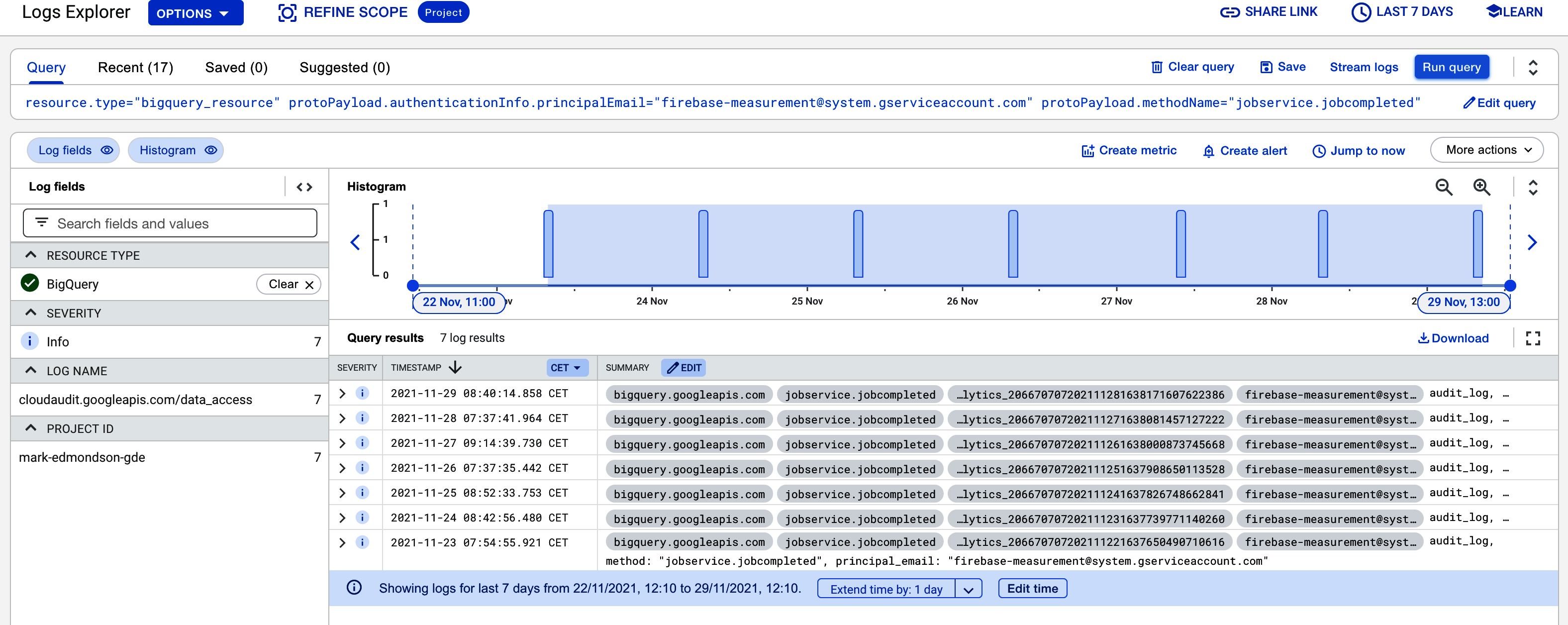
Figure 4-2. A Cloud Logging filter for seeing when your GA4 BigQuery exports are ready, which we can use to create a Pub/Sub topic

Once you’re happy with the log filter, select the “Logs Router” to route them into Pub/Sub. An example of the set-up screen is shown in Figure 4-3.

Once the log is created, you should get a Pub/Sub message each time the BigQuery export is ready for consumption later on. I suggest using Cloud Build to process the data, as detailed more in “Cloud Build”, or following the example in the next section, which will create a BigQuery partitioned table.

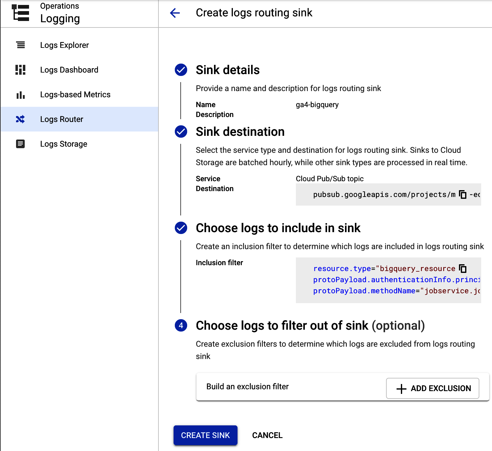
Figure 4-3. Setting up your GA4 BigQuery log so it sends the entries to Pub/Sub topic named ga4-bigquery

Creating Partitioned BigQuery Tables from Your GA4 Export

By default, the GA4 exports are in “sharded” tables, which means that each table is created separately and you use wildcards in the SQL to fetch them all, e.g., three days’ tables are called events_20210101, events_20210102, and events_20210103, which you can query via the SQL snippet SELECT * FROM dataset.events_*—the * is the wildcard.

This works, but if you wish to optimize your downstream queries, then aggregating the tables into one partitioned table will make some jobs flow easier and will allow some query optimizations for speed. We’ll use the Pub/Sub topic set up in Figure 4-3 to trigger a job that will copy the table over into a partitioned table.

To do this, go to the Pub/Sub topic and create a Cloud Function to be triggered by it by hitting the button at the top. The code to copy the table over into a partitioned table is in Example 4-5.

Example 4-5. Python code for a Cloud Function to copy your GA4 BigQuery exports into a partitioned table

import logging
import base64
import JSON
from google.cloud import bigquery # pip google-cloud-bigquery==1.5.1
import re

# replace with your dataset
DEST_DATASET = 'REPLACE_DATASET'

def make_partition_tbl_name(table_id):
  t_split = table_id.split('_20')

  name = t_split[0]

  suffix = ''.join(re.findall("\d\d", table_id)[0:4])
  name = name + '$' + suffix

  logging.info('partition table name: {}'.format(name))

  return name


def copy_bq(dataset_id, table_id):
  client = bigquery.Client()
  dest_dataset = DEST_DATASET
  dest_table = make_partition_tbl_name(table_id)

  source_table_ref = client.dataset(dataset_id).table(table_id)
  dest_table_ref = client.dataset(dest_dataset).table(dest_table)

  job = client.copy_table(
    source_table_ref,
    dest_table_ref,
    location = 'EU') # API request

  logging.info(f"Copy job:
   dataset {dataset_id}: tableId {table_id} ->
   dataset {dest_dataset}: tableId {dest_table} -
   check BigQuery logs of job_id: {job.job_id}
   for status")

def extract_data(data):
  """Gets the tableId, datasetId from pub/sub data"""
  data = JSON.loads(data)
  complete = data['protoPayload']['serviceData']['jobCompletedEvent']['job']
  table_info = complete['jobConfiguration']['load']['destinationTable']
  logging.info('Found data: {}'.format(JSON.dumps(table_info)))
  return table_info

def bq_to_bq(data, context):
  if 'data' in data:
    table_info = extract_data(base64.b64decode(data['data']).decode('utf-8'))
    copy_bq(dataset_id=table_info['datasetId'], table_id=table_info['tableId'])
  else:
    raise ValueError('No data found in pub-sub')

Deploy the Cloud Function with its own service account, and give that service account BigQuery Data Owner permissions. If possible, try to restrict to as specific a dataset or table as you can as a best practice.

Once the Cloud Function is deployed, your GA4 BigQuery exports will be duplicated into a partitioned table in another dataset. The Cloud Function reacts to the Pub/Sub message that the GA4 export is ready and triggers a BigQuery job to copy the table. This is helpful for applications such as the Data Loss Prevention API, which does not work with sharded tables, and is shown in an example application in “Data Loss Prevention API”.

Server-side Push to Pub/Sub

Another use for Pub/Sub is as part of your data collection pipeline if using GTM SS. From your GTM SS container, you can push all the event data to a Pub/Sub endpoint for use later.

Within GTM SS, you can create a container that will send all the event data to an HTTP endpoint. That HTTP endpoint can be a Cloud Function that will transfer it to a Pub/Sub topic—code to do that is shown in Example 4-6.

Example 4-6. Some example code to show how to send the GTM SS events to an HTTP endpoint, which will convert it into a Pub/Sub topic

const getAllEventData = require('getAllEventData');
const log = require("logToConsole");
const JSON = require("JSON");
const sendHttpRequest = require('sendHttpRequest');

log(data);

const postBody = JSON.stringify(getAllEventData());

log('postBody parsed to:', postBody);

const url = data.endpoint + '/' + data.topic_path;

log('Sending event data to:' + url);

const options = {method: 'POST',
         headers: {'Content-Type':'application/JSON'}};

// Sends a POST request
sendHttpRequest(url, (statusCode) => {
 if (statusCode >= 200 && statusCode < 300) {
  data.gtmOnSuccess();
 } else {
  data.gtmOnFailure();
 }
}, options, postBody);

A Cloud Function can be deployed to receive this HTTP endpoint with the GTM SS event payload and create a Pub/Sub topic, as shown in Example 4-7.

Example 4-7. An HTTP Cloud Function pointed to within the GTM SS tag that will retrieve the GTM SS event data and create a Pub/Sub topic with its content

import os, JSON
from google.cloud import pubsub_v1 # google-cloud-Pub/Sub==2.8.0

def http_to_Pub/Sub(request):
  request_JSON = request.get_JSON()
  request_args = request.args

  print('Request JSON: {}'.format(request_JSON))

  if request_JSON:
    res = trigger(JSON.dumps(request_JSON).encode('utf-8'), request.path)
    return res
  else:
    return 'No data found', 204


def trigger(data, topic_name):
 publisher = Pub/Sub_v1.PublisherClient()

 project_id = os.getenv('GCP_PROJECT')
 topic_name = f"projects/{project_id}/topics/{topic_name}"

 print ('Publishing message to topic {}'.format(topic_name))

 # create topic if necessary
 try:
  future = publisher.publish(topic_name, data)
  future_return = future.result()
  print('Published message {}'.format(future_return))

  return future_return

 except Exception as e:
  print('Topic {} does not exist? Attempting to create it'.format(topic_name))
  print('Error: {}'.format(e))

  publisher.create_topic(name=topic_name)
  print ('Topic created ' + topic_name)

  return 'Topic Created', 201

Firestore

Firestore is a NoSQL database as opposed to the SQL you may use in products such as “BigQuery”. As a complement for BigQuery, Firestore (or Datastore) is a counterpart that focuses on fast response times. Firestore works via keys that are used for quick lookups of data associated with it—and by quick, we mean subsecond. This means you must work with it in a different way than with BigQuery; most of the time, requests to the database should refer to a key (like a user ID) that returns an object (such as user properties).

Note

Firestore used to be called Datastore and is a rebranding of the product. Taking the best of Datastore and another product called Firebase Realtime Database, Firestore is a NoSQL document database built for automatic scaling, high performance, and ease of application development.

Firestore is linked to the Firebase suite of products and is usually used for mobile applications that need first lookups with mobile support via caching, batching, etc. Its properties can also be helpful for analytics applications because it’s ideal for fast lookups when giving an ID, such as a user ID.

When to Use Firestore

I typically use Firestore when I’m looking at creating APIs that will possibly be called multiple times per second, such as serving up a user’s attributes when given their user ID. This is usually more to support the data activation end of a project, with a light API that will take your ID, query the Firestore, and return with the attributes all within a few microseconds.

If you ever need a fast lookup, then Firestore will also be handy. An example that is powerful for analytics tracking is to keep your products database in a products Firestore with a lookup on the product SKU that returns that product’s cost, brand, category, etc. With such a database in place, you can improve your analytics collection by trimming down the ecommerce hits to include only the SKU and look up the data before sending it to GA4. This allows you to send much smaller hits from the user’s web browser with security, speed, and efficiency benefits.

Accessing Firestore Data Via an API

To access Firestore, you first need to import your data into a Firestore instance. You can do this via its import APIs or even by manually inputting via the WebUI. The requirement of the dataset is that you will always have a key that will be typically what you send to the database to return data, and then a nested JSON structure of data will come back.

Adding data to Firestore involves defining the object you want to record that could be in a nested structure and its location in the database. Altogether this defines a Firestore document. An example of how this would be added via Python is shown in Example 4-8.

Example 4-8. Importing a data structure into Firestore using the Python SDK, in this case, a demo product SKU with some details

from google.cloud import firestore
db = firestore.Client()

product_id = u'SKU12345'

data = {
  u'name': u'Muffins',
  u'brand': u'Mule',
  u'price': 15.78
}

# Add a new doc in collection 'your-firestore-collection'
db.collection(u'your-firestore-collection').document(product_id).set(data)

Using this means that you may need an additional data pipeline for importing your data into Firebase so that you can look up the data from your applications, which would use code similar to that in Example 4-8.

Once you have your data in Firestore, you can then reach it via your application. Example 4-9 gives a Python function you can use in a Cloud Function or App Engine application. We assume it’s being used to look up product information when it’s supplied a product_id.

Example 4-9. An example of how to read data from a Firestore database using Python within a Cloud Function

# pip google-cloud-firestore==2.3.4
from google.cloud import firestore

def read_firestore(product_id):
 db = firestore.Client()
 fs = 'your-firestore-collection'
 try:
  doc_ref = db.collection(fs).document(product_id)
 except:
  print(f'Could not connect to firestore collection: {fs}')
  return {}

 doc = doc_ref.get()
 if doc.exists:
  print(f'product_id data found: {doc.to_dict()}')
  return doc.to_dict()
 else:
  print(f'Could not find entry for product_id: {product_id}')
  return {}

Firestore gives you another tool that can help your digital analytics workflows and will come more to the fore when you need real-time applications and millisecond response times, such as calling from an API or as a user browses your website and you don’t want to add latency to their journey. It’s more suited to web application frameworks than to data analysis tasks, so it’s often used during the last steps of data activation.

BigQuery and Firestore are both examples of databases that work with structured data, but you’ll also come across unstructured data such as videos, pictures, or audio or just data you don’t know the shape of before you process it. In that case, your storage options need to work on a more low level of storing bytes, and that is where Cloud Storage comes into the picture.

GCS

We’ve already talked about using GCS for ingesting data into CRM systems in “Google Cloud Storage”, but this section is more about its use generally. GCS is useful for several roles, helped by the simple task it excels at: keeping bytes secure but instantly available.

GCS is the GCP service storage system most like the hard drive storing the files sitting on your computer. You can’t manipulate or do anything to that data until you open it up in an application, but it will store TBs of data for you to access in a secure and accessible manner. The roles I use it for are the following:

Unstructured data

For objects that can’t be loaded into a database such as video and images, GCS is a location that will always be able to help. It can store anything within bytes in its buckets, objects that are affectionately known as “blobs.” When working with Google APIs such as speech-to-text or image recognition, the files usually need to be uploaded to GCS first.

Raw data backups

Even for structured data, GCS is helpful as a raw data backup that can be stored at its archival low rates so you can always rewind or disaster-recover your way back from an outage.

Data import landing pads

As seen in “Google Cloud Storage”, GCS is helpful as a landing pad for export data since it won’t be fussy about the data schema or format. Since it will also trigger Pub/Sub events when data does arrive, it can start the event-based data flow systems.

Hosting websites

You can choose to make files publicly available from HTTP endpoints, meaning if you place HTML or other files supported by web browsers, you can have static websites hosted in GCS. This can also be helpful for static assets you may wish to import into websites such as for tracking pixels or images.

Dropbox

You can give public or more fine-grained access to certain users so you can securely pass on large files. Up to 5 TBs per object is supported, with unlimited (if you’re prepared to pay!) overall storage. This makes it a potential destination for data processing, such as a CSV file made available to colleagues who wish to import it locally into Excel.

Items stored in GCS are all stored at their own URI, which is like an HTTP address (https://example.com) but with its own protocol: gs://. You can also make them available at a normal HTTP address—in fact, you could host HTML files and GCS would serve as your web hosting.

The bucket names you use are globally unique, so you can access them from any project even if that bucket sits in another. You can specify public access over HTTP or only specific users or service emails working on behalf of your data applications. Figure 4-4 shows an example of how this looks via the WebUI, but the files within are usually accessed via code.

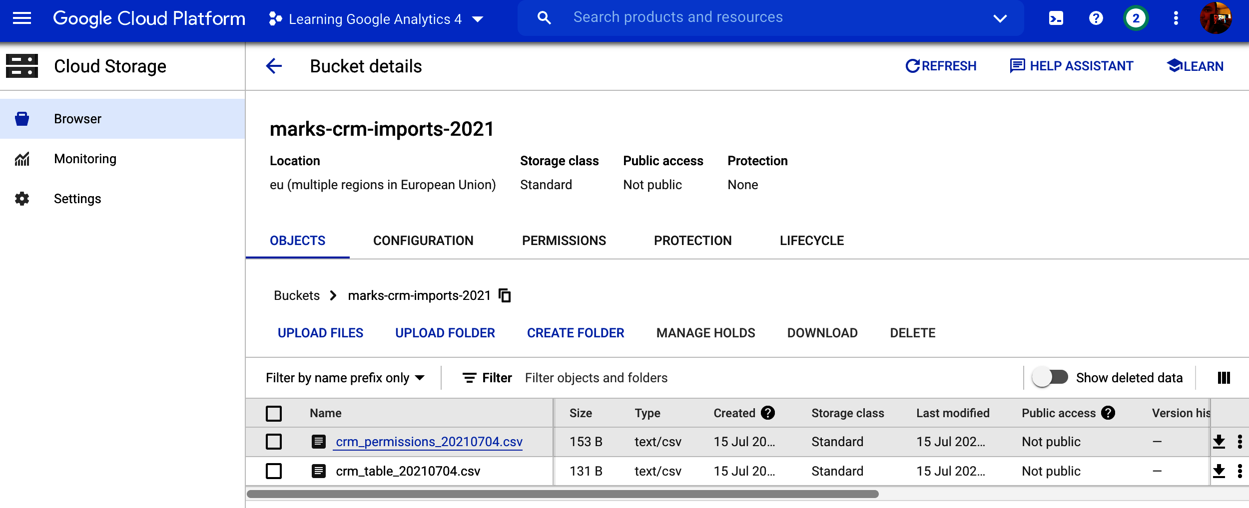
Figure 4-4. Files sitting within GCS in its WebUI

Each object in GCS has some metadata associated with it that you can use to tailor it to your storage needs. We’ll walk through the example file shown in Figure 4-5 to help illustrate what is possible.

Figure 4-5. Various metadata associated with a file upload to GCS

The metadata available for each object within GCS includes:

Type

This is an HTTP MIME (Multipurpose Internet Mail Extensions) type as specified for web objects. Mozilla’s website has some resources on HTTP MIME types. It’s worth setting this if your application will check against it to determine how to treat the file—for instance, a .csv file with MIME type text/csv in Figure 4-5 means applications downloading it will attempt to read it as a table. Other common MIME types you may come across are JSON (application/JSON), HTML for web pages (text/html), images such as image/png, and video (video/mp4).

Size

The size on disk of the object’s bytes. You can store up to 5 TB per object.

Created

When the object was first created.

Last modified

You can update objects by calling them the same name as when you first created them, and have object versioning activated.

Storage class

The pricing model that object is stored under, set at the bucket level. The storage classes are generally a compromise between storage cost and access cost. The costs for storage vary per region, but as a guide, here are some examples for GBs per month. Standard is for data that is accessed frequently ($0.02), Nearline for data that may be accessed a only few times a year ($0.01), Coldline for data that may be accessed only annually or less ($0.004), and Archive for data that may never be accessed aside from disaster recovery ($0.0012). Make sure to put your objects in the right class, or you will end up overpaying for data access because object cost prices are higher for accessing Archive data than for Standard, for example.

Custom time

You may have important dates or times to associate with the object, which you can add as metadata here.

Public URL

If you choose to make your object public, the URL will be listed here. Note that this is different from the Authenticated URL.

Authenticated URL

This is the URL if you’re giving restricted, not public, access to a user or application. It will check against that user’s authorization before serving up the object.

gstuil URI

The gs:// form of accessing the object, most typically when using it programmatically via the API or one of GCS’s SDKs.

Permission

Information about who can access the object. It’s typical these days for permission to be granted on a bucket level, although you can also choose to fine-grain control objects access. It’s usually easier to have two separate buckets for access control, such as public and restricted.

Protection

There are various methods you can enable to control how the object persists, which are highlighted in this section.

Hold status

You can enforce temporary or event-based holds on the object, meaning it can’t be deleted or modified when in place, either by a time limit or when a certain event triggered by an API call happens. This can be helpful to protect against accidental deletion, or if, for example, you have a data expiration active on the bucket via a retention policy but want to keep certain objects out of that policy.

Version history

You can enable versioning on your object such that even if it is modified, the older version will still be accessible. This can be helpful to keep a track record of scheduled data.

Retention policy

You can enable various rules that determine how long an object sticks around. This is vital if you’re dealing with personal user data to delete old archives once you no longer have permission to hold that data. You can also use it to move data into a lower-cost storage solution if it isn’t accessed after a certain number of days.

Encryption type

By default, Google operates an encryption approach to all your data on GCP, but you may want to enforce a tighter security policy in which not even Google can see the data. You cam do this by using your own security keys.

GCS is singular in purpose, but it’s a fundamental purpose: store your bytes safely and securely. It is the bedrock that several other GCP services rely on, even if they’re not exposed to the end user and can serve that role for you too. It’s an infinite hard drive in the cloud rather than on your own computer, and it can be easily accessed across the world.

We’ve now looked at the three major data storage types: BigQuery for structured SQL data, Firestore for NoSQL data, and GCS for unstructured raw data. We now turn to how you work with them on a regular basis, looking at techniques for scheduling and streaming data flows. Let’s start with the most common application, scheduled flows.

Scheduling Data Imports

This section looks at one of the major tasks for any data engineer designing workflows: how to schedule data flows within your applications. Once your proof of concept is working, your next step to putting that into production is being able to regularly update the data involved. Rather than updating a spreadsheet each day or running an API script, turning this task over to the many automation devices available to you on GCP ensures that you will have continuously updated data without needing to worry about it.

There are many ways to approach data updates, which this section will go through in relation to how you want to move your GA4 data and its companion datasets.

Data Import Types: Streaming Versus Scheduled Batches

Streaming data versus batching data is one of those decisions that you may come across when designing data application systems. This section considers some of the advantages and disadvantages of both.

Streaming data flows are more real time, using event-based small data packets that are continuously being updated. Batched data is regularly scheduled at a slower interval, such as daily or hourly, with larger data imports each job.

The streaming options for data will be considered more in depth in “Streaming Data Flows”, but comparing them side by side with batched data can help with some fundamental decisions early on in your application design.

Batched data flows

Batching is the most common and traditional way of importing data flows, and for most use cases it’s perfectly adequate. A key question when creating your use case will be how fast you need that data. It’s common for the initial reaction to be as fast as possible or near real time. But looking at the specifics, you find that actually the effects of hourly or even daily updates will be unnoticeable compared to real time, and these types of updates will be a lot cheaper and easier to run. If the data you’re updating with is also batched (for example, a CRM export that happens nightly), there will be little reason to make downstream data real time. As always, look at the use case application and see if it makes sense. Batched data workflows start to break down if you can’t rely on those scheduled updates to be on time. You may then need to create fallback options if an import fails (and you should always design for eventual failure).

Streaming data flows

Streaming data is easier to do these days in modern data stacks given the new technologies available, and there are proponents who will say all your data flows should be streaming if possible. It may well be that you discover new use cases once you break free from the shackles of batched data schedules. There are certain advantages even if you’re not in immediate need of real-time data since when moving to an event-based model of data we react when something happens, not when a certain timestamp is reached, which means we can be more flexible in when data flows occur. A good example of this is the GA4 BigQuery data exports, which if delayed would break downstream dashboards and applications. Setting up event-based reactions to when the data is available means you will get the data as soon as it’s there, rather than having to wait for the next day’s delivery. The major disadvantage is cost because these flows are typically more expensive to run. Your data engineers will also need a different skill level to be able to develop and troubleshoot streaming pipelines.

When considering scheduled jobs, we’ll start with BigQuery’s own resources, then branch out into more sophisticated solutions such as Cloud Composer, Cloud Scheduler, and Cloud Build.

BigQuery Views

In some cases, the simplest way to present transformed data is to set up a BigQuery View or schedule BigQuery SQL. This is the easiest to set up and involves no other services.

BigQuery Views are not tables in the traditional sense but rather represent a table that would result from the SQL you use to define it. This means that when you create your SQL, you can include dynamic dates and thus always have the latest data. For example, you could be querying your GA4 BigQuery data exports with a View created as in Example 4-10—this will always bring yesterday’s data back.

Example 4-10. This SQL can be used in a BigQuery View to always show yesterday’s data (adapted from Example 3-6)

SELECT
  -- event_date (the date on which the event was logged)
  parse_date('%Y%m%d',event_date) as event_date,
  -- event_timestamp (in microseconds, utc)
  timestamp_micros(event_timestamp) as event_timestamp,
  -- event_name (the name of the event)
  event_name,
  -- event_key (the event parameter's key)
  (SELECT key FROM UNNEST(event_params)
   WHERE key = 'page_location') as event_key,
  -- event_string_value (the string value of the event parameter)
  (SELECT value.string_value FROM UNNEST(event_params)
   WHERE key = 'page_location') as event_string_value
FROM
  -- your GA4 exports - change to your location
  `learning-ga4.analytics_250021309.events_*`
WHERE
  -- limits query to use table from yesterday only
  _TABLE_SUFFIX = FORMAT_DATE('%Y%m%d',date_sub(current_date(), INTERVAL 1 day))
  -- limits query to only show this event
  and event_name = 'page_view'

The key line is FORMAT_DATE('%Y%m%d',date_sub(current_date(), INTERVAL 1 day)), which returns yesterday, which takes advantage of the _TABLE_SUFFIX column BigQuery adds as meta information about the table so that you can more easily query multiple tables.

BigQuery Views have their place, but be careful using them. Since the View SQL is running underneath any other queries run against them, you can run into expensive or slow results. This has been recently mitigated with Materialized Views, which is a technology to make sure you don’t query against the entire table when making queries on top of Views. In some cases, you may be better off creating your own intermediate table, perhaps via a scheduler to create the table, which we cover in the next section.

BigQuery Scheduled Queries

BigQuery has native support for scheduling queries, accessible via the menu bar at the top left or by selecting “Schedule” when you create the query. This is fine for small jobs and imports; I would, however, caution against relying on this for anything other than single-step, simple transformations. Once you’re looking at more complicated data flows, then it will become easier to use dedicated tools for the job, both from a management and robustness perspective.

Scheduled queries are tied to the user authentication who sets them up, so if that person leaves, the scheduler will need to be updated via the gcloud command bq update --transfer-config --update-credentials. Perhaps use this to update your connection to service accounts that are not linked to one person. You’ll also have only the BigQuery Scheduler interface to control the queries—for large complicated queries you want to modify, this will make it hard to see a change history or overview.

But for simple, nonbusiness-critical queries that are needed perhaps for a limited number of people, it is quick and easy to set up within the interface itself, and it would serve better than Views for, say, exports to dashboard solutions such as Looker or Data Studio. As seen in Figure 4-6, once you have developed your SQL and have results you like, you can hit the “Schedule” button and have the data ready for you when you log in the next day.

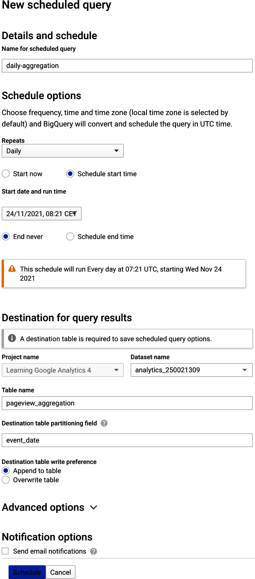
Figure 4-6. Setting up a scheduled query from Example 4-10, which may perform better than creating a BigQuery View with the same data for use in dashboards, etc.

However, once you start asking questions like, “How can I make this scheduled query more robust?” or “How can I trigger off queries based on the data I’m creating in this table?” this is a sign you will need a more robust solution for scheduling. The tool for that job is Airflow, via its hosted version on GCP called Cloud Composer that we talk about in the next section.

Cloud Composer

Cloud Composer is a Google-managed solution for Airflow, a popular open source scheduling tool. It costs around $300 a month, so it’s only worth looking at once you have some good business value to justify it, but it is the solution I trust the most when looking at complicated data flows across multiple systems, offering backfilling, alerting systems, and configuration via Python. Many companies consider it the backbone of all of their scheduling jobs.

Note

I will use the name Cloud Composer in this book since that is what managed Airflow is called within the GCP, but a large amount of the content will be applicable to Airflow running on other platforms as well, such as other cloud providers or self-hosted platform.

I started to use Cloud Composer once I had jobs that fulfilled the following criteria:

Multilevel dependencies

As soon as you have a situation in your data pipelines where one scheduled job depends on another, I would start using Cloud Composer since it will fit well within its directed acyclic graph (DAG) structure. Examples include chains of SQL jobs: one SQL script to tidy the data, another SQL script to make your model data. Putting these SQL scripts to be executed within Cloud Composer allows you to break up your scheduled jobs into smaller, simpler components than if try to run them all in one bigger job. Once you have the freedom to set dependencies, I recommend improving pipelines by adding checks and validation steps that would be too complex to do via a single scheduled job.

Backfills

It’s common to set up a historic import at the start of the project to backfill all the data you would have had if the schedule job was running, for example, the past 12 months. What is available will differ per job, but if you have set up imports per day it can sometimes be nontrivial to then set up historic imports. Cloud Composer runs jobs as a simulation of the day, and you can set any start date so it will slowly backfill all data if you let it.

Multiple interaction systems

If you’re pulling in data or sending data to multiple systems such as FTP, Cloud products, SQL databases, and APIs, it will start to become complex to coordinate across those systems and may require spreading them out across various import scripts. Cloud Composer’s many connectors via its Operators and Hooks means it can connect to virtually anything, so you can manage them all from one place, which is a lot easier to maintain.

Retries

As you import over HTTP, in a lot of cases, you will experience outages. It can be difficult to configure when and how often to retry those imports or exports, which Cloud Composer can help with via its configurable retry system that controls each task.

Once working with data flows, you will quickly experience issues like the ones mentioned and need a way to solve them easily, for which Cloud Composer is one solution. Similar solutions exist, but Cloud Composer is the one I’ve used the most and has quickly become the backbone of many data projects. How to represent these flows in an intuitive manner is useful to be able to imagine complicated processes, which Cloud Composer solves using a representation we talk about next.

DAGs

The central feature of Cloud Composer are DAGs, which represent the flow of your data as it is ingested, processed, and extracted. The name refers to a node and edge structure, with directions between those nodes given by arrows. An example of what that could mean for your own GA4 pipeline is shown in Figure 4-7.

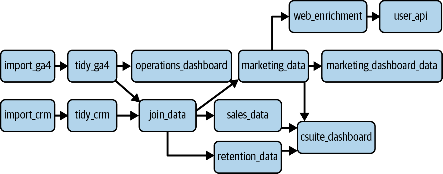
Figure 4-7. An example of a DAG that could be used in a GA4 process

The nodes represent a data operation, with the edges showing the order of events and which operations are dependent on one another. One of the key features of Airflow is that if one node fails (which eventually all do), then it has strategies in place to either wait, retry, or skip downstream operations. It also has some backfill features that can prevent a lot of headaches from running historic updates, and it comes with some predefined macros that allow you to dynamically insert, for example, today’s date into your scripts.

An example of a DAG that imports from your GA4 BigQuery exports is shown in Example 4-11.

Example 4-11. An example DAG that takes your GA4 export and aggregates it using SQL that you have developed earlier and in a ga4-bigquery.sql file uploaded with your script

from airflow.contrib.operators.bigquery_operator import BigQueryOperator
from airflow.contrib.operators.bigquery_check_operator import BigQueryCheckOperator
from airflow.operators.dummy_operator import DummyOperator
from airflow import DAG
from airflow.utils.dates import days_ago
import datetime

VERSION = '0.1.7' # increment this each version of the DAG

DAG_NAME = 'ga4-transformation-' + VERSION

default_args = {
  'start_date': days_ago(1), # change this to a fixed date for backfilling
  'email_on_failure': True,
  'email': '[e-mail]',
  'email_on_retry': False,
  'depends_on_past': False,
  'retries': 3,
  'retry_delay': datetime.timedelta(minutes=10),
  'project_id': 'learning-ga4',
  'execution_timeout': datetime.timedelta(minutes=60)
}

schedule_interval = '2 4 * * *' # min, hour, day of month, month, day of week

dag = DAG(DAG_NAME, default_args=default_args, schedule_interval=schedule_interval)


start = DummyOperator(
  task_id='start',
  dag=dag
)

# uses the Airflow macro {{ ds_nodash }} to insert todays date in YYYYMMDD form
check_table = BigQueryCheckOperator(
  task_id='check_table',
  dag=dag,
  sql='''
  SELECT count(1) > 5000
  FROM `learning-ga4.analytics_250021309.events_{{ ds_nodash }}`"
  '''
)

checked = DummyOperator(
  task_id='checked',
  dag=dag
)

# a function so you can loop over many tables, SQL files
def make_bq(table_id):

  task = BigQueryOperator(
    task_id='make_bq_'+table_id,
    write_disposition='WRITE_TRUNCATE',
    create_disposition='CREATE_IF_NEEDED',
    destination_dataset_table=
        'learning_ga4.ga4_aggregations.{}${{ ds_nodash}}'.format(table_id),
    sql='./ga4_sql/{}.sql'.format(table_id),
    use_legacy_sql=False,
    dag=dag
  )

  return task

ga_tables = [
 'pageview-aggs',
 'ga4-join-crm',
 'ecom-fields'
]

ga_aggregations = [] # helpful if you are doing other downstream transformations
for table in ga_tables:
 task = make_bq(table)
 checked >> task
 ga_aggregations.append(task)


# create the DAG
start >> check_table >> checked

To make the nodes for your DAG, you will use Airflow Operators, which are various functions premade to connect to a variety of applications, including an extensive GCP array of services such as BigQuery, FTP, Kubernetes clusters, and so on.

For the example in Example 4-11, the nodes are created by:

start

A DummyOperator() to signpost the start of the DAG.

check_table

A BigQueryCheckOperator() that will check that you have data that day in the GA4 table. If this fails by returning FALSE for the inline SQL shown, Airflow will fail the task and retry it again every 10 minutes up to 3 times. You can modify this to your expectations.

checked

Another DummyOperator() to signpost that the table has been checked.

make_bq

This will create or add to a partitioned table with the same name as the task_id. The SQL it will execute should also have the same name and be available in the SQL folder uploaded with the DAG, in ./ga4_sql/, e.g., ./ga4_sql/pageview-aggs.sql. It is functionalized so you can loop over tableIds for more efficient code.

The edges are taken care of via bitwise Python operators at the end of the tag and within the loops, e.g., start >> check_table >> checked.

You can see the resulting DAG displayed in Figure 4-8. Take this example as a basis you can expand for your own workflows.

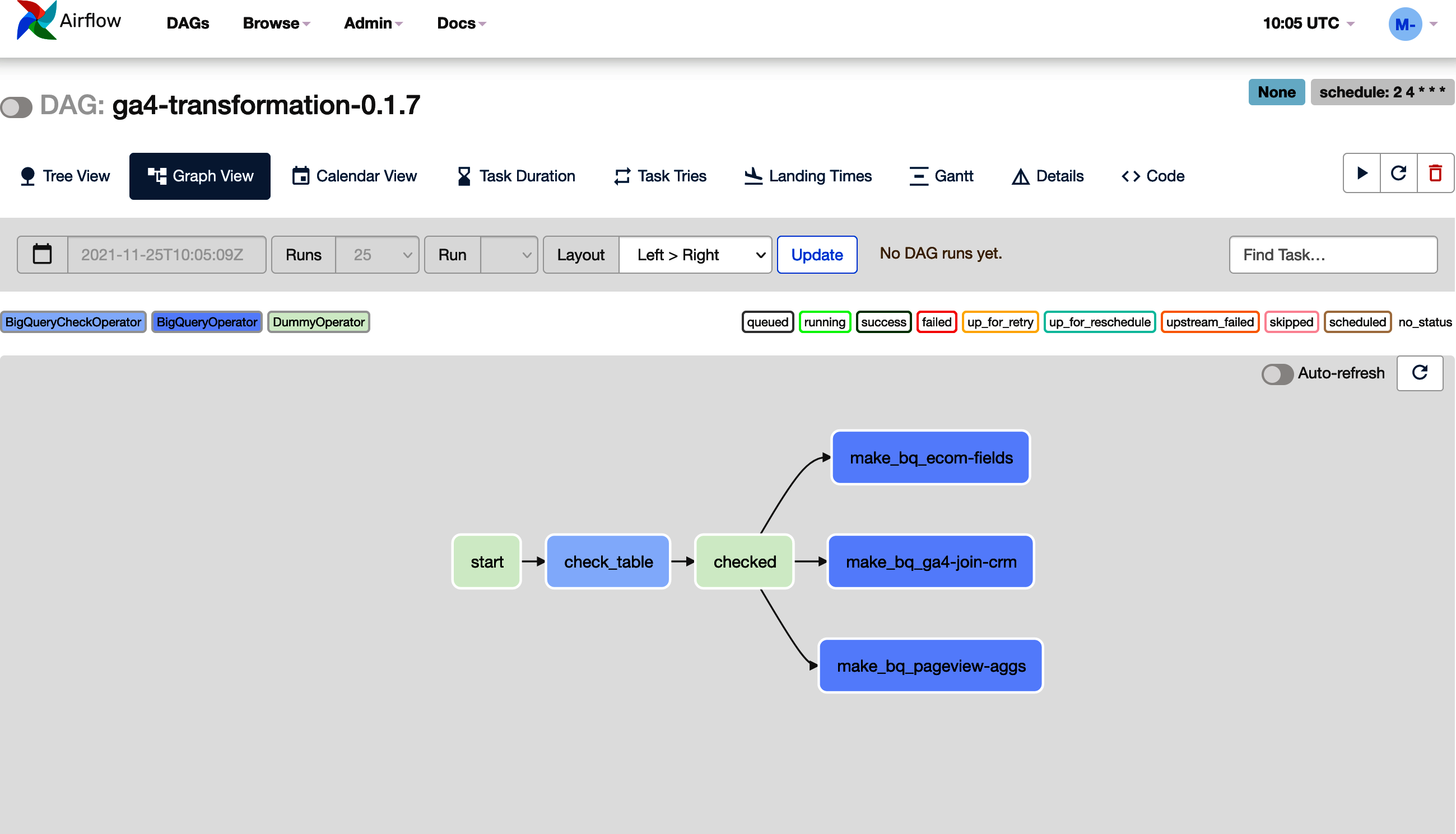
Figure 4-8. An example of the DAG created in Airflow by the code in Example 4-11; to scale up for more transformations, add more SQL files to the folder and add the name of the table to the ga_tables list

Tips for using Airflow/Cloud Composer

The general help files are excellent for learning how to use Cloud Composer, but the following are some tips I’ve picked up while using it within data science projects:

Use Airflow only for scheduling

Use the right tool for the right job—Airflow’s role is scheduling and connecting to data storage systems. I made the mistake of using its Python libraries to massage data a bit between scheduling steps but got into a Python dependency hell that affected all running tasks. I prefer to use Docker containers for any code that needs to run, and use the GKEPodOperator() instead to run that code in a controlled environment.

Write functions for your DAGS

It’s much cleaner to create functions that output DAGs rather than having the tasks written out each time. It also means you can loop over them and create dependencies for lots of datasets at once without needing to copy-paste code.

Use dummy operators to signpost

The DAGs look impressive but can be confusing, so having some handy signposts along the line can indicate where you can stop and start misbehaving DAG runs. Being able to clear all downstream from “Data all loaded” signpost makes it clear what will happen. Other features that can help here are Task Groups and Labels, which can help display meta information about what your DAG is doing.

Separate out your SQL files

You don’t have to write out huge strings of SQL for your operators; you can instead put them into .sql files and then call the file holding the SQL. This makes it much easier to track and keep on top of changes.

Version your DAG names

I also find it helpful to increment the version of the DAG name as you modify and update. Airflow can be a bit slow in recognizing new updates to files, so having the version name in the DAG means you can be sure you’re always working on the latest version.

Set up Cloud Build to deploy DAGs

Having to upload your DAG code and files each time will disincentivize you to make changes, so it’s much easier if you set up a Cloud Build pipeline that will deploy your DAGs upon each commit to GitHub.

That was a flying tour of Cloud Composer features, but there is a lot more to it, and I recommend the Airflow website to explore more of its options. It is a heavyweight scheduling option, and there is another, much lighter, option in Google Cloud Scheduler, which we’ll look at next.

Cloud Scheduler

If you’re looking for something more lightweight than Cloud Composer, then Cloud Scheduler is a simple cron-in-the-cloud service you can use to trigger HTTP endpoints. For simple tasks that don’t need the complexity of data flows supported by Cloud Composer, it just works.

I put it somewhere in between Cloud Composer and BigQuery-scheduled queries in capabilities, since Cloud Scheduler will run not just BigQuery queries but any other GCP service as well since that can be handy.

To do that, it does involve some extra work to create the Pub/Sub topic and Cloud Function that will create the BigQuery job, so if it’s just BigQuery, you may not have a need, but if other GCP services are involved, centralizing the location of your scheduling may be better in the long run. You can see an example of setting up a Pub/Sub topic in “Pub/Sub”; the only difference is that then you schedule an event to hit that topic via Cloud Scheduler. You can see some examples from my own GCP in Figure 4-9 that shows the following:

Packagetest-build

A weekly schedule to trigger an API call to run a Cloud Build

Slackbot-schedule

A weekly schedule to hit an HTTP endpoint that will trigger a Slackbot

Target_Pub/Sub_scheduler

A daily schedule to trigger a Pub/Sub topic

Figure 4-9. Some Cloud Schedules I enabled for some tasks within my own GCP

Cloud Scheduler can also trigger other services such as Cloud Run or Cloud Build. A particularly powerful combination is Cloud Scheduler and Cloud Build (covered in the next section, “Cloud Build”). Since Cloud Build can run long-running tasks, you have an easy way to create a serverless system that can run any job on GCP, all event-driven but with some scheduling on top.

Cloud Build

Cloud Build is a powerful tool to consider for data workflows, and it’s probably the tool I use most every day (even more than BigQuery!). Cloud Build was also introduced in the data ingestion section in “Setting Up Cloud Build CI/CD with GitHub”, but we’ll go into more detail here.

Cloud Build is classified as a CI/CD tool, which is a popular strategy in modern-day data ops. It mandates that code releases to production should not be at the end of massive development times but with little updates all the time, with automatic testing and deployment features so that any errors are quickly discovered and can be rolled back. These are good practices in general, and I encourage reading up on how to follow them. Cloud Build can also be thought of as a generic way to trigger any code on a compute cluster in reaction to events. The primary intention is for when you commit code to a Git repository such as GitHub, but those events could also be when a file hits GCS, a Pub/Sub message is sent, or a scheduler pings the endpoint.

Cloud Build works by you defining the sequences of events, much like an Airflow DAG but with a simpler structure. For each step, you define a Docker environment to run your code within, and the results of that code running can be passed on to subsequent steps or archived on GCS. Since it works with any Docker container, you can run a multitude of different code environments on the same data; for instance, one step could be Python to read from an API, then R to parse it out, then Go to send the result someplace else.

I was originally introduced to Cloud Build as the way to build Docker containers on GCP. You place your Dockerfile in a GitHub repository and then commit, which will trigger a job and build Docker in a serverless manner, and not on your own computer as you would normally. This is the only way I build Docker containers these days, as building them locally takes time and a lot of hard disk space. Building in the cloud usually means committing code, going for a cup of tea, and then coming back in 10 minutes to inspect the logs.

Cloud Build has now been extended to building not only Dockerfiles but also its own YAML configuration syntax (cloudbuild.yaml) as well as buildpacks. This greatly extends its utility because, via the same actions (Git commit, Pub/Sub event, or a schedule), you can trigger off jobs to do a whole variety of useful tasks, not just Docker containers but running any code you require.

I’ve distilled the lessons I’ve learned from working with Cloud Build along with the HTTP Docker equivalent Cloud Run and Cloud Scheduler into my R package googleCloudRunner, which is the tool I use to deploy most of my data engineering tasks for GA4 and otherwise on GCP. Cloud Build uses Docker containers to run everything. I can run almost any language/program or application, including R. Having an easy way to create and trigger these builds from R means R can serve as a UI or gateway to any other program, e.g., R can trigger a Cloud Build using gcloud to deploy Cloud Run applications.

Cloud Build configurations

As a quick introduction, a Cloud Build YAML file looks something like that shown in Example 4-12. The example shows how three different Docker containers can be used within the same build, doing different things but working on the same data.

Example 4-12. An example of a cloudbuild.yaml file used to create builds. Each step happens sequentially. The name field is of a Docker image that will run the command specified in the args field.

steps:
- name: 'gcr.io/cloud-builders/docker'
 id: Docker Version
 args: ["version"]
- name: 'alpine'
 id: Hello Cloud Build
 args: ["echo", "Hello Cloud Build"]
- name: 'rocker/r-base'
 id: Hello R
 args: ["R", "-e", "paste0('1 + 1 = ', 1+1)"]

You then submit this build using the GCP web console, gcloud or googleCloudRunner, or otherwise using the Cloud Build API. The gcloud version is gcloud builds submit --config cloudbuild.yaml --no-source. This will trigger a build in the console where you can watch it via its logs or otherwise—see Figure 4-10 of an example for the googleCloudRunner package checks:

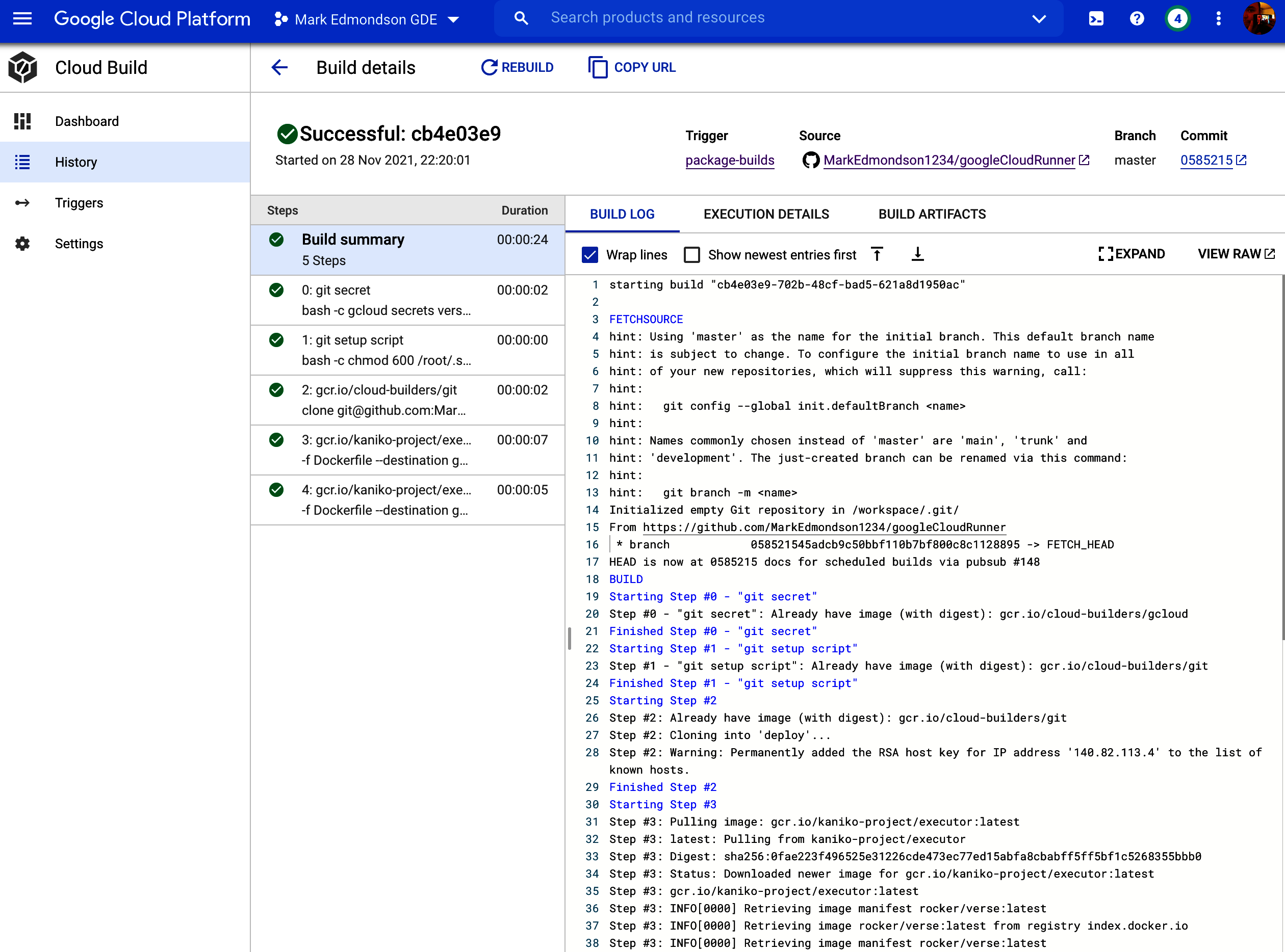
Figure 4-10. A Cloud Build that has successfully built within the Google Cloud Console

We’ve also seen Cloud Build used to deploy a Cloud Function in “Setting Up Cloud Build CI/CD with GitHub”—that example is replicated in Example 4-13. Only one step is needed to deploy the Cloud Function from Example 3-9.

Example 4-13. Cloud Build YAML for deploying a Cloud Function from Example 3-9

steps:
- name: gcr.io/cloud-builders/gcloud
 args: ['functions',
     'deploy',
     'gcs_to_bq',
     '--runtime=python39',
     '--region=europe-west1',
     '--trigger-resource=marks-crm-imports-2021',
     '--trigger-event=google.storage.object.finalize']

Builds can be triggered manually, but often you want this to be an automatic process, which starts to embrace the CI philosophy. For those, you use Build Triggers.

Build Triggers

Build Triggers is a configuration that decides when your Cloud Build will fire. You can set up Build Triggers to react to Git pushes, Pub/Sub events, or webhooks only when you manually fire them in the console. The build can be specified in a file or inline within the Build Trigger configuration. We’ve already covered how to set up Build Triggers in “Setting Up the GitHub Connection to Cloud Build”, so see that section for a walk-through.

We covered Cloud Build in general, but we now move to a specific example for GA4.

GA4 applications for Cloud Build

In general, I deploy all code for working with GA4 data through Cloud Build, since it’s linked to the GitHub repository I put my code within when not working in the GA4 interface. That covers Airflow DAGs, Cloud Functions, BigQuery tables, etc., via various Cloud Build steps invoking gcloud, my R libraries, or otherwise.

When processing the standard GA4 BigQuery exports, Cloud Logging creates an entry showing when those tables are ready, which you can then use to create a Pub/Sub message. This can kick off an event-driven data flow such as invoking an Airflow DAG, running SQL queries, or otherwise.

An example follows where we’ll create a Cloud Build that will run from the Pub/Sub topic triggered once your GA4 BigQuery exports are present. In “Setting Up a Pub/Sub Topic for GA4 BigQuery Exports”, we created a Pub/Sub topic called “ga4-bigquery,” which fires each time the exports are ready. We’ll now consume this message via a Cloud Build.

Create a Build Trigger that will respond to the Pub/Sub message. An example is shown in Figure 4-11. For this demonstration, it will read a cloudbuild.yml file that is within the code-examples GitHub repo. This repo contains the work you wish to do on the BigQuery export for that day.

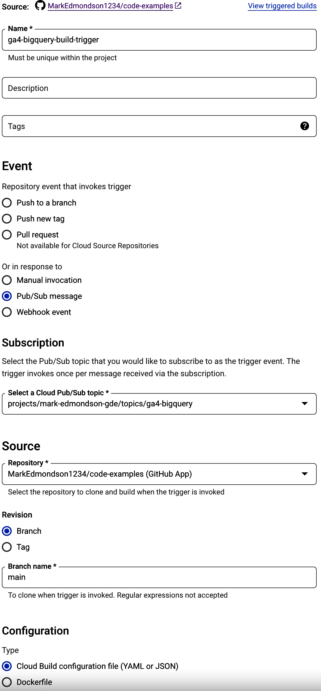
Figure 4-11. Setting up a Build Trigger that will build once the BigQuery export for GA4 is complete

Now we need the build that the Build Trigger will kick off when it gets that Pub/Sub message. We’ll adapt the example from Example 4-10 and put this in an SQL file. This is committed to the GitHub source, which the Build will clone before executing. This will allow you to adapt the SQL easily by committing up to GitHub.

Example 4-14. The build the Build Trigger will do when it gets the Pub/Sub event from the GA4 BigQuery export completion; the SQL from Example 4-10 is uploaded in a separate file called ga4-agg.sql

steps:
- name: 'gcr.io/cloud-builders/gcloud'
 entrypoint: 'bash'
 dir: 'your/dir/on/Git'
 args: ['-c',
     'bq --location=eu \
     --project_id=$PROJECT_ID query \
     --use_legacy_sql=false \ --destination_table=tidydata.ga4_pageviews \
     < ./ga4-agg.sql']

To run Example 4-14 successfully, the user permissions need to be adjusted to allow authorized use to carry out the query. This will not be your own user, since the job will be done on your behalf by the Cloud Build service agent. Within your Cloud Build settings or in the Google Console you will find the service user who will carry out the commands within the Cloud Build, which will look something like [e-mail]. You can use this, or you can create your own custom service account with Cloud Build permissions. This user needs to be added as a BigQuery Admin so they can carry out queries and other BigQuery tasks, such as creating tables, that you may want later. See Figure 4-12.

For your own use cases, you will need to adapt the SQL and perhaps add more steps to work with the data once this step is complete. You can see that Cloud Build is serving a similar role as Cloud Composer but in a simpler way. It’s more generic than scheduling queries in BigQuery but not as expensive or feature-rich as Cloud Composer; I find it a nice tool in the toolbox for when you need simple tasks to be scheduled or event-driven.

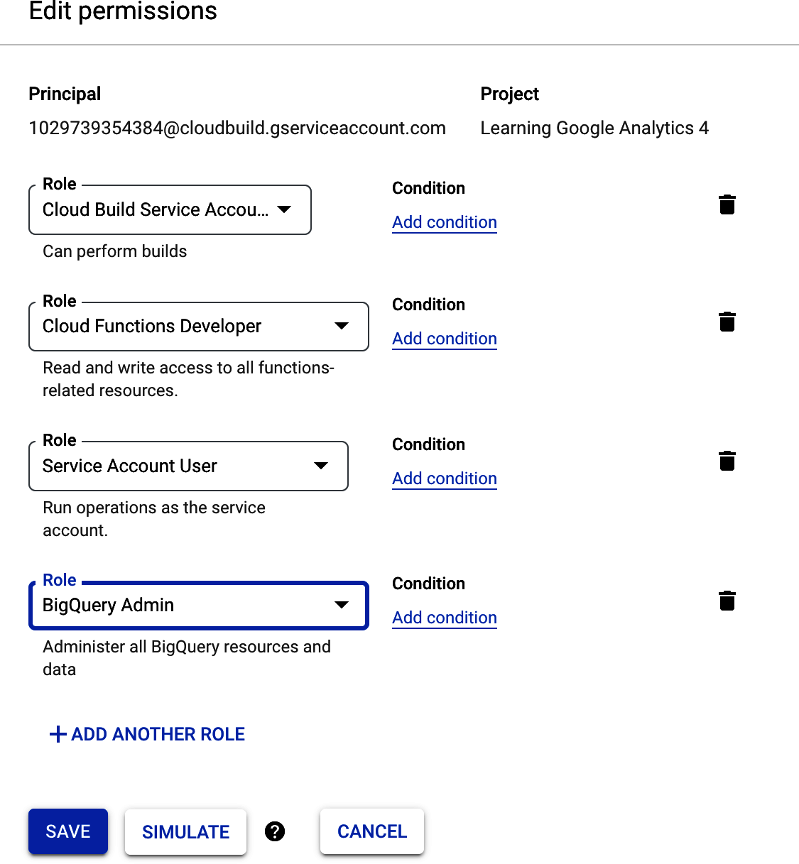
Figure 4-12. Adding the permissions to execute BigQuery jobs to the Cloud Build service account

Cloud Build integrations for CI/CD

Cloud Build can be triggered via schedules, manual invocations, and events. The events cover Pub/Sub and GitHub commits, which are key to its role as a CI/CD tool. In general, it’s a good idea when coding to use version control such as Git, and I use GitHub, the most popular version. This way you can keep a record of everything you do and also have an infinite undo to roll back changes if you need to—and when the difference between success and failure can be a . in the wrong place, then this is desirable!

Once you’re using Git for version control, you can then also start using it for other purposes, such as triggering builds off of each commit to check your code (tests), make sure it follows style guidelines (linting), or trigger actual builds of the product the code creates.

Cloud Build allows any code language within it via its use of Docker containers, which are used to control the environments of each step. It also features easy authentication for Google Cloud service via gcloud auth, as we saw in Figure 4-12, when setting it up to make BigQuery tasks. The gcloud commands that you use to deploy services can also be used within Cloud Build to automate those deployments. In addition, all the execution can be based off the code you are committing to the Git repository, so you will have a perfect overview of what is happening and when.

For example, we can deploy DAGs to Airflow, as was done in Example 4-11. Normally, to have your DAG deploy, you need to copy that Python file into a special folder within the Cloud Composer environment, but with Cloud Build you can use gsutil (the GCS command-line tool) to do it instead. This encourages more rapid development and gives you some time back to focus on the important things. An example of the cloudbuild file for your trigger is shown in Example 4-15.

Example 4-15. You can deploy python DAGs for Airflow/Cloud Composer using Cloud Build straight from your Git repository—​here $_AIRFLOW_BUCKET is a substitution variable you change to the location of your installation, and the .sql files are assumed to be within a folder named sql in the same location

steps:
- name: gcr.io/google.com/cloudsdktool/cloud-sdk:alpine
 id: deploy dag
 entrypoint: 'gsutil'
 args: ['mv',
     'dags/ga4-aggregation.py',
     '$_AIRFLOW_BUCKET/dags/ga4-aggregation.py']
- name: gcr.io/google.com/cloudsdktool/cloud-sdk:alpine
 id: remove old SQL
 entrypoint: 'gsutil'
 args: ['rm',
     '-R',
     '${_AIRFLOW_BUCKET}/dags/sql']
- name: gcr.io/google.com/cloudsdktool/cloud-sdk:alpine
 entrypoint: 'gsutil'
 id: add new SQL
 args: ['cp',
     '-R',
     'dags/sql',
     '${_AIRFLOW_BUCKET}/dags/sql']

Similar to the previous example for Cloud Composer, Cloud Build can be used to deploy for all other GCP services as well. We use it again in Example 3-15 to deploy Cloud Functions, but any service that uses a gcloud command can be automated.

Batched data scheduling services are usually core to all data applications, including those involving GA4. We’ve taken a tour through some of your options when looking at scheduling, including BigQuery scheduled queries, Cloud Scheduler, Cloud Build, and Cloud Composer/Airflow. Each have the following advantages and disadvantages:

BigQuery scheduled queries

Easy to set up but lack accountability and work only for BigQuery

Cloud Scheduler

Works for all services, but complicated dependencies will start to become hard to maintain

Cloud Build

Event-based and can trigger from schedules, usually my preferred choice, but does not support flows that need backfills and retries

Cloud Composer

Comprehensive scheduling tool with backfills, support for complicated work-flows, and retry/service level agreement (SLA) features but the most expensive and complicated to work with

Hopefully, this has given you some ideas about what you could use for your own use cases. In the next section, we look at more real-time data flows and the tools you may use when you need to process your data immediately.

Streaming Data Flows

For some workflows, batched scheduling may not be enough. If you’re looking for reactive data updates under half an hour, for example, it may be time to start looking at the streaming data flow options. Several of the solutions share some of the same features and components, but there is an increased cost and complexity that comes with real-time streaming data that you need to factor in.

Pub/Sub for Streaming Data

The examples up to now have only treated Pub/Sub with relatively low data volumes, just events to say something has happened. However, its main purpose is for dealing with high-volume data streams, and this is where it really shines. It’s at-least-once delivery system means you can build reliable data flows even if you’re putting TBs worth of data through it. In fact, Googlebot, the search engine bot that built up Google Search, also runs on a similar infrastructure, and it regularly downloads the entire internet so you know Pub/Sub can scale!

The support for streaming data will most likely start with Pub/Sub as the entry point that other streaming systems send data toward from Kafka or other on-premises systems. When setting up these real-time ingestions, it’s usually the internal application developers that will set up this stream before handing it off once they want that stream to flow into the GCP. This is usually where I get involved, with my responsibility being to help define the schema of data coming into the Pub/Sub topic and then taking it onward from there.

Once you have data flowing into a Pub/Sub topic, it has out-of-the-box solutions to start streaming that to popular destinations, such as Cloud Storage and BigQuery. These are provided by Apache Beam or the Google-hosted version, Dataflow.

Apache Beam/DataFlow

The go-to service for streaming data around GCP is Dataflow. Dataflow is a service that runs jobs written in Apache Beam, a data processing library that started off in Google but is now available open source, so you can also use it as a standard for other clouds.

Apache Beam works by creating virtual machines (VMs) with Apache Beam installed that are set up to execute code that will operate on each data packet as it flows in. It has autoscaling built in, so if the machine’s resources begin to get stretched (i.e., thresholds on CPU and/or memory are hit), then it will launch another machine and route some of the traffic to that. It will cost more or less depending on how much data you’re sending in, with a minimum floor of 1 VM.

There are common data jobs that are expedited for Apache Beam by its templates. For example, a common task is to stream Pub/Sub into BigQuery, which is available without having to write any code at all. An example is shown in Figure 4-13.

To work with the template, you will need to create a bucket and the BigQuery table the Pub/Sub messages will flow into. The BigQuery table needs to have the correct schema that should match the Pub/Sub data schema.

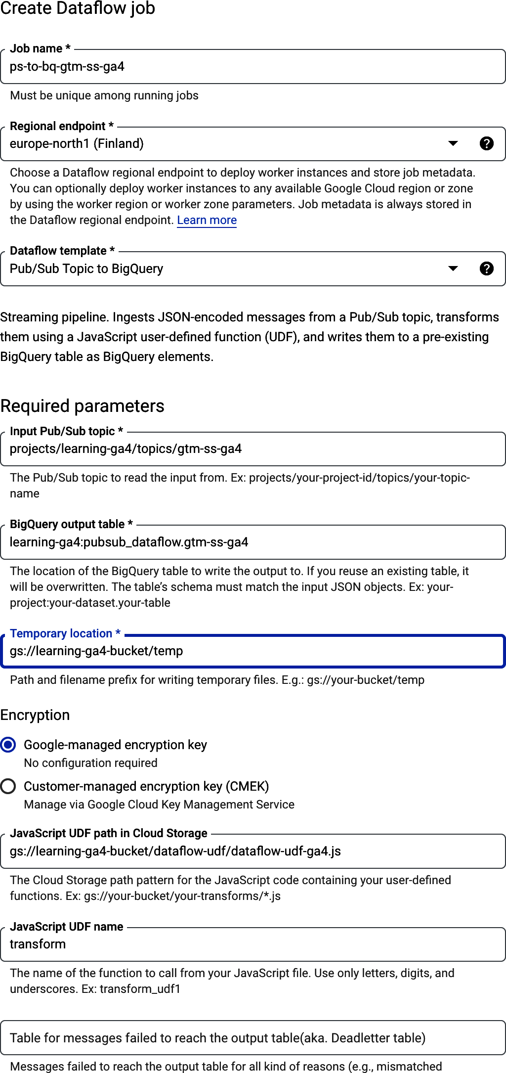
Figure 4-13. Setting up a Dataflow from within the Google Cloud Console for a Pub/Sub topic into BigQuery via the predefined template

For my example, I’m streaming in some GA4 events from my blog into Pub/Sub via GTM SS (see “Streaming GA4 events into Pub/Sub with GTM SS”). By default, the stream will attempt to write every Pub/Sub field to a BigQuery table, and your BigQuery schema will need to match exactly to succeed. This can be problematic if your Pub/Sub includes fields that are invalid in BigQuery, such as those with hyphens (-) that are present in Example 4-16.

Example 4-16. An example of the JSON sent from a GA4 tag in GTM SS to Pub/Sub, which has some fields starting with x-ga

{"x-ga-protocol_version":"2",
"x-ga-measurement_id":"G-43MXXXX",
"x-ga-gtm_version":"2reba1",
"x-ga-page_id":1015778133,
"screen_resolution":"1536x864",
"language":"ru-ru",
"client_id":"68920138.12345678",
"x-ga-request_count":1,
"page_location":"https://code.markedmondson.me/data-privacy-gtm/",
"page_referrer":"https://www.google.com/",
"page_title":"Data Privacy Engineering with Google Tag Manager Server Side and ...",
"ga_session_id":"12343456",
"ga_session_number":1,
"x-ga-mp2-seg":"0",
"event_name":"page_view",
"x-ga-system_properties":{"fv":"2","ss":"1"},
"debug_mode":"true",
"ip_override":"78.140.192.76",
"user_agent":"Mozilla/5.0 (Windows NT 10.0; Win64; x64) AppleWebKit/537.36 ...",
"x-ga-gcs-origin":"not-specified",
"user_id":"123445678"}

To accommodate your customization needs, you can supply a transformation function that will modify the stream before it passes it into BigQuery. For example, we can filter out the fields that start with x-ga.

The Dataflow user-defined function (UDF) in Example 4-17 filters out those events, so the rest of the template can send the data into BigQuery. This UDF needs to be uploaded to a bucket for the Dataflow workers to download and use it.

Example 4-17. A Dataflow user-defined function that filters out Pub/Sub topic fields starting with x-ga so the rest of the data can be written to BigQuery

/**
 * A transform function that filters out fields starting with x-ga
 * @param {string} inJSON
 * @return {string} outJSON
 */
 function transform(inJSON) {
  var obj = JSON.parse(inJSON);
  var keys = Object.keys(obj);
  var outJSON = {};

  // don't output keys that starts with x-ga
  var outJSON = keys.filter(function(key) {
    return !key.startsWith('x-ga');
  }).reduce(function(acc, key) {
    acc[key] = obj[key];
    return acc;
  }, {});

  return JSON.stringify(outJSON);
 }

Once the Dataflow job is set up, it will give you a DAG much like Cloud Composer/Airflow, but in this system it will be dealing with real-time event-based flows, not batches. Figure 4-14 shows what you should see in your Dataflow Jobs section in the web console.

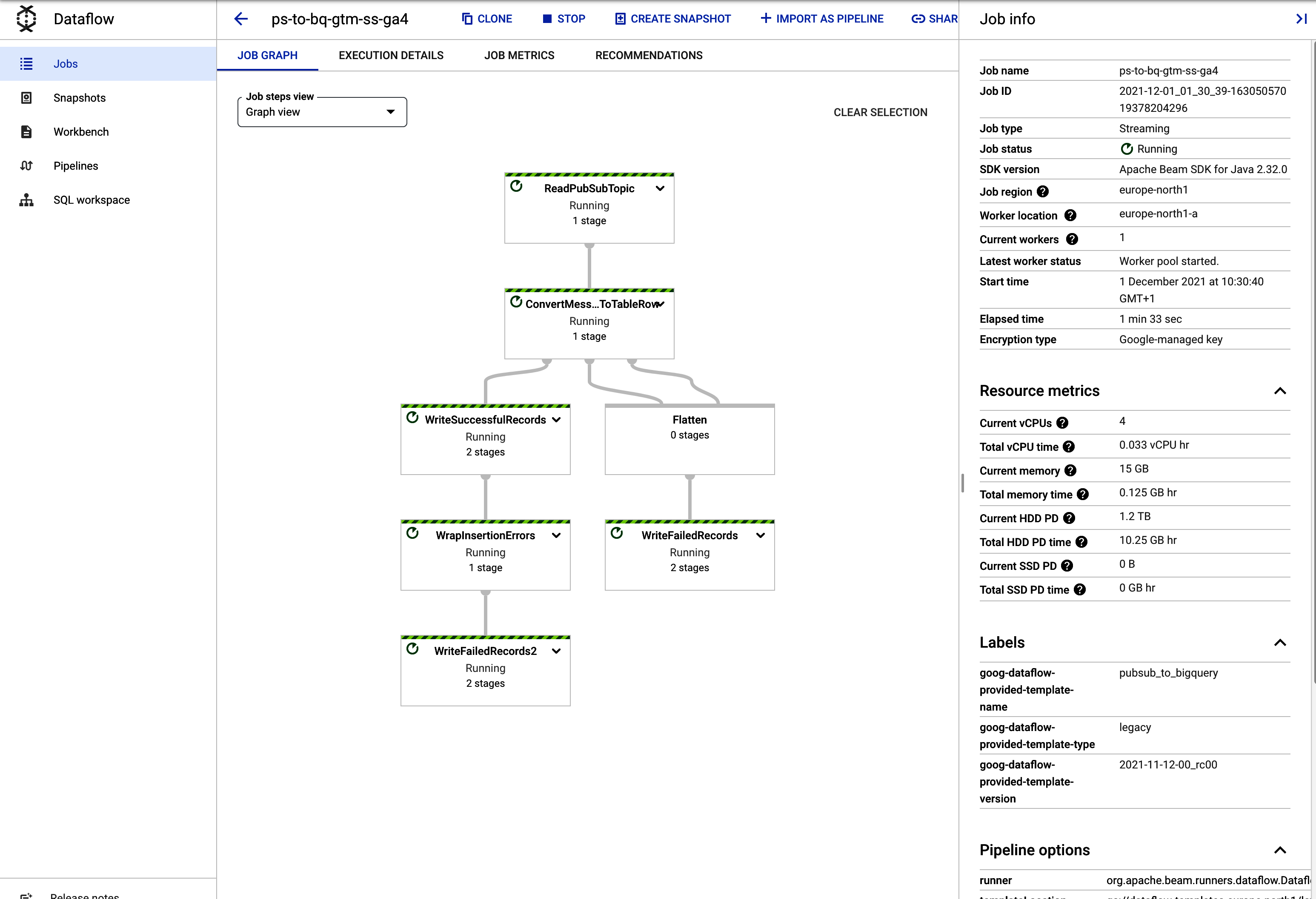
Figure 4-14. Starting up a running job for importing Pub/Sub messages into BigQuery in real time

Costs of Dataflow

Given the way Dataflow works, be wary of spinning up too many VMs because if you get an error, that can send a lot of hits into your pipeline, and you can quickly run up expensive bills. Once you have an idea of your workload, it’s wise to set an upper limit on the VMs to deal with the spikes of data but not let it run away from you if something really unexpected happens. Even with these precautions, the solution is still more expensive than batched workflows, since you can expect to spend in the region of $10 to $30 a day or $300 to $900 a month.

The BigQuery schema needs to match the Pub/Sub configuration, so we need to create a table. The table in Figure 4-15 is also set up to be time partitioned.

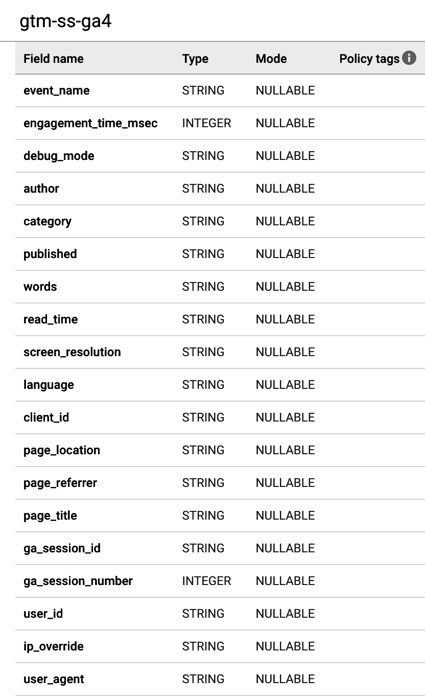
Figure 4-15. The BigQuery data schema to receive the Pub/Sub JSON

If you make any mistakes, the Dataflow job will stream the raw data into another table in the same dataset where you can examine the errors and make corrections, as shown in Figure 4-16.

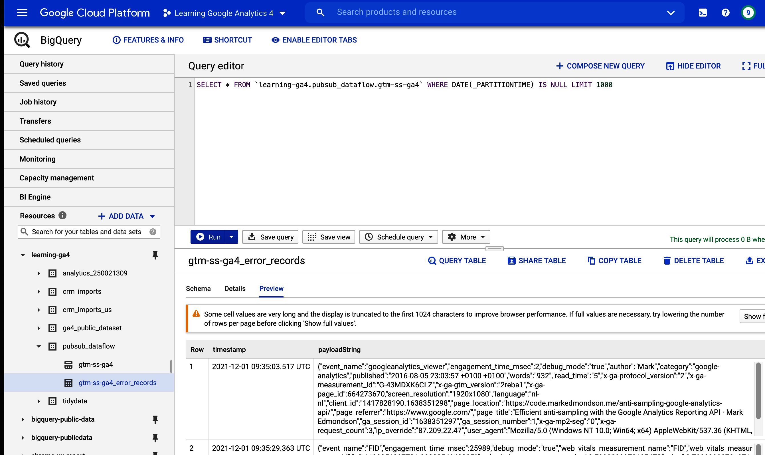
Figure 4-16. Any errors from the Dataflow will appear in its own BigQuery table so you can examine the payloads

If everything is going well, you should see your Pub/Sub data start to appear in BigQuery—give yourself a pat on the back if you see something similar to Figure 4-17.

A standard BigQuery export functionality is already available to you for free by using GA4’s native BigQuery exports, but this process can be adapted for other use cases directing to different endpoints or making different transformations. An example may be to work with a subset of your GA4 events to modify the hit to be more privacy aware or to enrich it with product metadata available only via another real-time stream.

Remember that Dataflow will be running a VM at an expense for this flow, so turn it off if you don’t need it. If your data volumes aren’t large enough to warrant such an expense, you can also use Cloud Functions to stream data.

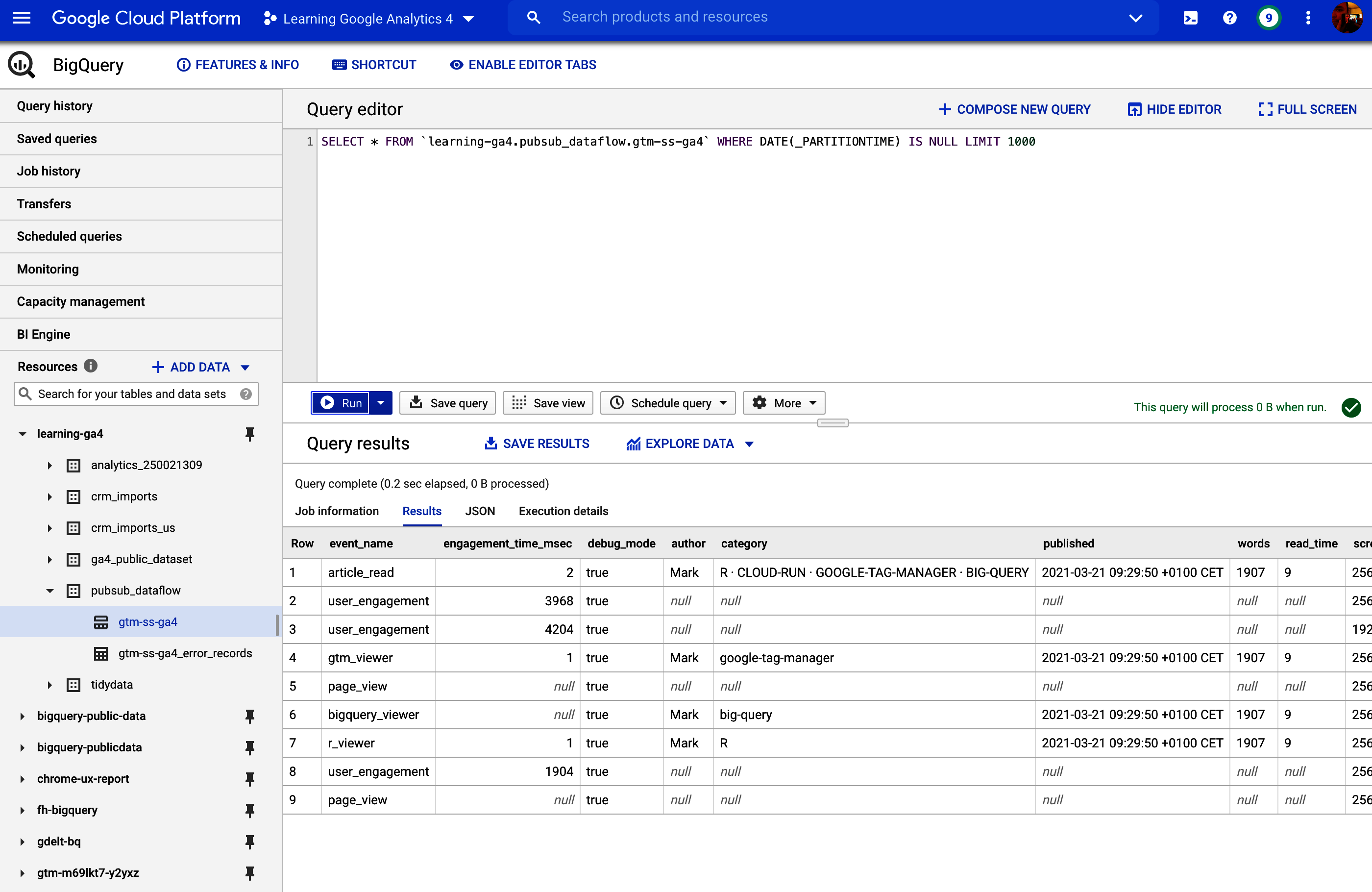
Figure 4-17. A successful streaming import from GA4 into GTM SS to Pub/Sub to BigQuery

Streaming Via Cloud Functions

If your data volumes are within Cloud Function quotas, your Pub/Sub topic setup can also use Cloud Functions to stream the data to different locations. Example 4-5 has some example code for sporadic events like BigQuery tables, but you can also react to more regular streams of data and Cloud Function will scale up and down as needed—each invocation of the Pub/Sub event will create a Cloud Function instance that will run in parallel with other functions.

Limits (for Generation 1 Cloud Functions) include only 540 seconds (9 minutes) of runtime and a total of 3,000 seconds of simultaneous invocations (e.g., if a function takes 100 seconds to execute, you can have up to 30 functions running at a time). This means you should make your Cloud Functions small and efficient.

The following Cloud Function should be small enough that you can have around 300 requests per second (Example 4-18). It takes the Pub/Sub message and puts it as a string into a raw data column in BigQuery along with its timestamp. You can modify the code to parse out more specific schema as you need it or use BigQuery SQL itself to process the raw JSON string into tidier data later.

Example 4-18. Modify the pb dict within the code to parse out more fields if you want to create a more bespoke table. Add environment arguments dataset and table pointing at your premade BigQuery table. Inspired by Milosevic’s Medium post about how to copy data from Pub/Sub to BigQuery.

# python 3.7
# pip google-cloud-bigquery==2.23.2
from google.cloud import bigquery
import base64, JSON, sys, os, time

def Pub/Sub_to_bigq(event, context):
  Pub/Sub_message = base64.b64decode(event['data']).decode('utf-8')
  print(Pub/Sub_message)
  pb = JSON.loads(Pub/Sub_message)
  raw = JSON.dumps(pb)

  pb['timestamp'] = time.time()
  pb['raw'] = raw
  to_bigquery(os.getenv['dataset'], os.getenv['table'], pb)

def to_bigquery(dataset, table, document):
  bigquery_client = bigquery.Client()
  dataset_ref = bigquery_client.dataset(dataset)
  table_ref = dataset_ref.table(table)
  table = bigquery_client.get_table(table_ref)
  errors = bigquery_client.insert_rows(table, [document], ignore_unknown_values=True)
  if errors != [] :
   print(errors, file=sys.stderr)

The function takes environment arguments to specify where the data goes, as shown in Figure 4-18. This enables you to deploy multiple functions for different streams.

The premade BigQuery table has only two fields, raw, which contains the JSON string, and timestamp, when the Cloud Function executed. You can use BigQuery’s JSON functions in SQL to parse out this raw JSON string, as shown in Example 4-19.

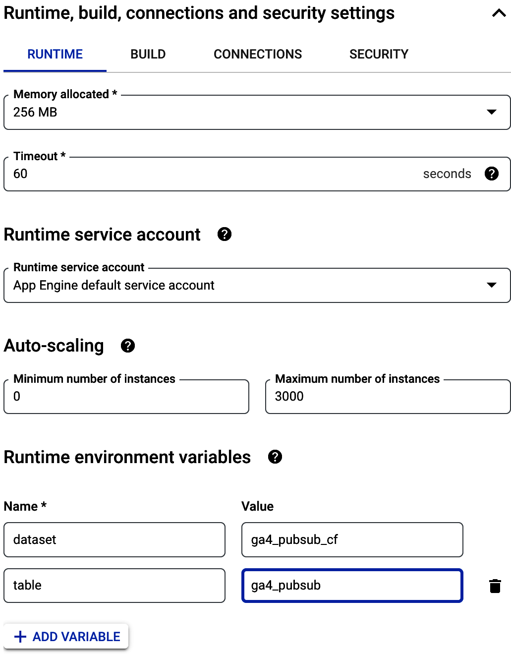
Figure 4-18. Setting the environment arguments for use within the Cloud Function in Example 4-18

Example 4-19. BigQuery SQL to parse out a raw JSON string

SELECT
 JSON_VALUE(raw, "$.event_name") AS event_name,
 JSON_VALUE(raw, "$.client_id") AS client_id,
 JSON_VALUE(raw, "$.page_location") AS page_location,
 timestamp,
 raw
FROM
 `learning-ga4.ga4_Pub/Sub_cf.ga4_Pub/Sub`
WHERE
 DATE(_PARTITIONTIME) IS NULL
LIMIT
 1000

The result of the code in Example 4-19 is shown in Figure 4-19. You can set up this SQL downstream in a schedule or via a BigQuery View.

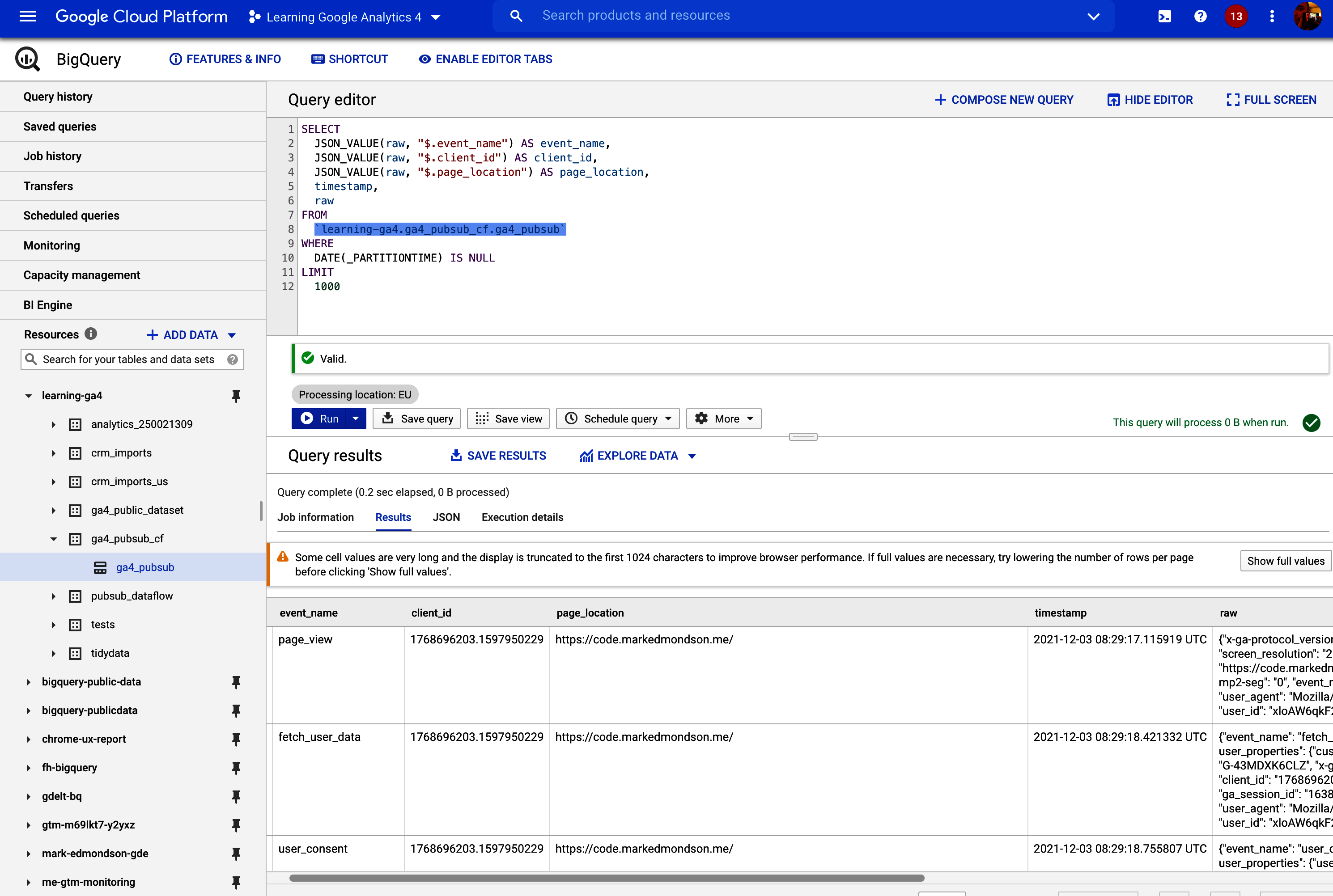
Figure 4-19. The raw data table receiving the Pub/Sub stream from GA4 via GTM-SS can have its JSON parsed out with BigQuery’s functions such as JSON_VALUE()

Streaming data services offer a way to have the most responsive and modern data stack for your GA4 set up but they do come at a financial and technological cost that you will need to justify with a great business case. However, if you have that case, having these tools available means you should be able to get something up and running, an application that would have been almost impossible to do 10 years ago.

Digital analytics data streams such as GA4 are usually the most useful when they can tailor experiences to an individual user, but when using data that can be associated with a person, you need to be extra mindful of the consequences both legally and ethically. We’ll delve into this in the next section.

Protecting User Privacy

“User Privacy” also gives an overview of user privacy, but this section goes into more depth and gives some technical resources.

In this modern data age, the value of data has been realized by those who are providing that data and not just by those using it. Taking that data without permission can now be regarded as immoral as theft, so to be a long-term sustainable business, it’s increasingly important to gain your users’ trust. The most trusted brands will be those that are clear on what data they are capturing and how they are using that data, as well as those that give users easy access to their own data, so much so that they have the ability to make informed choices, have the power to reclaim their own data, and take back permission to use it. Following on from these evolving ethics, the laws of various regions are also starting to become stricter and be more impactful, with the possibilty of heavy fines if you do not comply.

When storing data that can be traced back to an individual, you have a responsibility to protect that personal data from both internal abuse and external malignant actors who may try to steal it.

This section looks at data storage design patterns that will help you make the data privacy process easier. In some cases, noncompliance has occurred not by intent but by a poorly designed system, which we’ll look to prevent.

Data Privacy by Design

The easiest way to avoid data privacy concerns is to simply not store personal data. Unless you have a specific need for that personal data, removing it from your data capture or erasing it as it comes into storage is the easiest way to keep on top of it. This may sound flippant, but it does need to be stated, since it’s quite common for companies to just collect this data by accident or without really thinking about the consequences. A classic case with web analytics is accidentally storing user emails in the URLs for web forms or in search boxes. Even if accidental, this is against Google Analytics Terms of Service and carries the risk of having your account closed down. Having some data cleaning in place at the point of collection can go a long way toward keeping a clean house.

If you do need some level of personalization, you still need not necessarily capture data that will pose a privacy risk. This is where pseudonomyzation comes in, which is the default for data collection, including GA4. Here’s an ID is assigned to a user, but it is that ID that is shared, not the user’s personal data. An example is choosing between a random ID or a person’s phone number as a user ID. If the random ID is accidentally exposed, an attacker couldn’t do much with it unless they had access to the system that mapped that ID to the rest of that person’s information. If the ID exposed is actually a person’s phone number, the attacker has something they can use immediately. Using pseudonomyzation is a first line of defense for guarding a user’s personal data. Again, never use email or a phone number as an ID because you will run into privacy breaches; companies who have done this have been fined.

It may be that the ID is all you need for your use cases—for instance, the default GA4 data collection is at this level. Only when you start to link that ID to personal information, such as linking GA4’s client_id to a user’s email address, will you need to start considering more extreme privacy considerations. This typically happens when you start linking it to your backend systems like a CRM database.

Should your use cases then require personal data, email, name, or otherwise, there are some principles to keep in place, encouraged by privacy legislation such as GDPR. These steps will allow you to preserve the user’s dignity as well as have some business impact with that data:

Keep personal data (PII) in minimal number of locations

Personal data should be kept in as few databases as possible and then joined or linked to other systems via a pseudonymous ID that is the key for that table. This way you should only ever have one place to look if you need to delete or extract a person’s data, and you won’t need to also delete it from subsequent places it may have been copied or joined to. This complements the next point about encryption of user data, since you should only need to do that with the user database.

Encrypt user data with salt-and-peppered hashes

The process of hashing is a method of one-way encrypting data so that it is impossible to re-create the original data without knowing the ingredients: for instance, “Mark Edmondson” when hashed with the popular sha256 hashing algorithm is:

3e7e793f2b41a8f9c703898c5c0d4e08ab2f22aa1603f8d0f6e4872a8f542335

However, it is always this hash and should be globally unique so you can use it as a reliable key. To “salt and pepper” the hash means you also add a unique keyword to the data to make it even more secure should somehow someone break the hashing algorithm or can obtain the same hash to make a link. For instance, if my salt is “baboons,” then I prefix it to my data point so that “Mark Edmondson” becomes “baboonsMark Edmondson,” and the hash is:

a776b81a2a6b1c2fc787ea0a21932047b080b1f08e7bc6d6a2ccd1fb6443df48

e.g., completely different than before. Salts can be global or stored with the user point to make them unique for each user. To “pepper” or “secret salt” the hash is a similar concept, but this time the keyword is not kept alongside the data to encrypt but in another secure location. This guards against database breaches because it now has two locations. In this case, the “pepper” would be fetched and may be “averylongSECRETthatnoonecanknow?” and so my final hash will be “baboonsMark EdmondsonaverylongSECRETthatnoonecanknow?” to give a final hash of:

c9299fe251319ffa7ec66137acfe81c75ee115ceaa89b3e74b521a0b5e12d138

which should be very difficult for a motivated hacker to reidentify the user with.

Put data expiration times on personal data

Sometimes you will have no option but to copy personal data across, for instance, if you’re importing from different clouds or systems. In that case, you can nominate the data source as the source of truth for all your privacy initiatives and then enforce a data expiration date on any data that is copied from that source. Thirty days is typical, meaning you need to do a full import at least every 30 days (maybe even daily) so the data volumes will increase. You should then be secure knowing that as you update user permissions and values in your master database, any copies of that data will be ephemeral and not be around at all once the imports stop.

Adding privacy principles does add extra work, but the payoff is peace of mind and trust in your own systems, which can be conveyed to your customers. An example of the last point for data expiration within some of the storage systems we’ve talked about in this chapter is demonstrated in the next section.

Data Expiration in BigQuery

When setting up your datasets, tables, and buckets, you can set the data expiration for your data that is coming in. We’ve already covered how to set it in GCS in “Google Cloud Storage”.

For BigQuery, you can set an expiration date at the dataset level that will affect all tables within that dataset—see Figure 4-20 for an example with a test dataset.

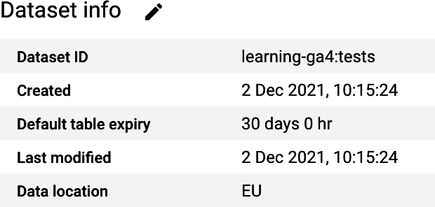
Figure 4-20. You can configure the table expiration time when you create a dataset

For partitioned tables, you will need something different, since the table will always exist but you want the partitions themselves to expire over time, leaving you with only the most recent data. For that, you will need to invoke gcloud or use the BigQuery SQL for altering table properties, as shown in Example 4-20.

Example 4-20. Setting a date expiration for BigQuery partitions in a partition table

The gcloud way (via your local bash console or in Cloud Console):

bq update --time_partitioning_field=event_date \
 --time_partitioning_expiration 604800 [PROJECT-ID]:[DATASET].partitioned_table

Or via BigQuery DML:

ALTER TABLE `project-name`.dataset_name.table_name
SET OPTIONS (partition_expiration_days=7);

As well as the passive data expiration times, you can also actively scan data for privacy breaches via the Data Loss Prevention API.

Data Loss Prevention API

The Data Loss Prevention (DLP) API is a way to automatically detect and mask sensitive data such as emails, phone numbers, and credit card numbers. You can call it and run it on your data within Cloud Storage or BigQuery.

If you have a large amount of streaming data, there is a Dataflow template available to read CSV data from GCS and put the redacted data into BigQuery.

For GA4, you can most easily use it to scan your BigQuery exports to see if any personal data has been collected inadvertently. The DLP API scans only one table at a time, so the best way to use this is to scan your incoming data table each day. If you have a lot of data, I recommended scanning only a sample and/or restrict the scan to only the fields that may contain sensitive data. For GA4 BigQuery exports in particular, this is most likely to be only the event_params.value.string_value since all other fields are more or less fixed by your configuration (event_name, etc.).

Summary

Because data comes in such a variety of forms and uses, there are many different systems available to hold it. The broad categories we have spoken about in this chapter are structured and unstructured data and scheduled versus streaming pipelines between those systems. You also need a good organizing structure with some thought on who and what should access each piece of data along its journey, since at the end of the day, it’s people who will be using that data, and lowering the friction for the right person to see the right data is a big step toward data maturity within your organization. As soon as you need data beyond GA4, you need to know how these systems interact, but you have a good starting point with the GA4 BigQuery exports, which is highly regarded as one of its key features over Universal Analytics.

Now that we’ve talked about how to collect and store data, in the next chapter, we’ll get more into how that data is actively massaged, transformed, and modeled, and how it usually represents where the most value is added within the pipeline.