Learning Data Science

Chapter 4. Modeling with Summary Statistics

We saw in Chapter 2 the importance of data scope and in Chapter 3 the importance of data generation mechanisms, such as one that can be represented by an urn model. Urn models address one aspect of modeling: they describe chance variation and ensure that the data are representative of the target. Good scope and representative data lay the groundwork for extracting useful information from data, which is the other part of modeling. This information is often referred to as the signal in the data. We use models to approximate the signal, with the simplest of these being the constant model, where the signal is approximated by a single number, like the mean or median. Other, more complex models summarize relationships between features in the data, such as humidity and particulate matter in air quality (Chapter 12), upward mobility and commute time in communities (Chapter 15), and height and weight of animals (Chapter 18). These more complex models are also approximations built from data. When a model fits the data well, it can provide a useful approximation to the world or simply a helpful description of the data.

In this chapter, we introduce the basics of model fitting through a loss formulation. We demonstrate how to model patterns in the data by considering the loss that arises from using a simple summary to describe the data, the constant model. We delve deeper into the connections between the urn model and the fitted model in Chapter 16, where we examine the balance between signal and noise when fitting models, and in Chapter 17, where we tackle the topics of inference, prediction, and hypothesis testing.

The constant model lets us introduce model fitting from the perspective of loss minimization in a simple context, and it helps us connect summary statistics, like the mean and median, to more complex modeling scenarios in later chapters. We begin with an example that uses data about the late arrival of a bus to introduce the constant model.

The Constant Model

A transit rider, Jake, often takes the northbound C bus at the 3rd & Pike bus stop in downtown Seattle.¹ The bus is supposed to arrive every 10 minutes, but Jake notices that he sometimes waits a long time for the bus. He wants to know how late the bus usually is. Jake was able to acquire the scheduled arrival and actual arrival times for his bus from the Washington State Transportation Center. From these data, he can calculate the number of minutes that each bus is late to arrive at his stop:

times = pd.read_csv('data/seattle_bus_times_NC.csv')
times

	route	direction	scheduled	actual	minutes_late
0	C	northbound	2016-03-26 06:30:28	2016-03-26 06:26:04	-4.40
1	C	northbound	2016-03-26 01:05:25	2016-03-26 01:10:15	4.83
2	C	northbound	2016-03-26 21:00:25	2016-03-26 21:05:00	4.58
...	...	...	...	...	...
1431	C	northbound	2016-04-10 06:15:28	2016-04-10 06:11:37	-3.85
1432	C	northbound	2016-04-10 17:00:28	2016-04-10 16:56:54	-3.57
1433	C	northbound	2016-04-10 20:15:25	2016-04-10 20:18:21	2.93

1434 rows × 5 columns

The minutes_late column in the data table records how late each bus was. Notice that some of the times are negative, meaning that the bus arrived early. Let’s examine a histogram of the number of minutes each bus is late:

fig = px.histogram(times, x='minutes_late', width=450, height=250)
fig.update_xaxes(range=[-12, 60], title_text='Minutes late')
fig

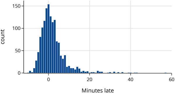
We can already see some interesting patterns in the data. For example, many buses arrive earlier than scheduled, but some are well over 20 minutes late. We also see a clear mode (high point) at 0, meaning many buses arrive roughly on time.

To understand how late a bus on this route typically is, we’d like to summarize lateness by a constant—this is a statistic, a single number, like the mean, median, or mode. Let’s find each of these summary statistics for the minutes_late column in the data table.

From the histogram, we estimate the mode of the data to be 0, and we use Python to compute the mean and median:

mean:    1.92 mins late
median:  0.74 mins late
mode:    0.00 mins late

Naturally, we want to know which of these numbers best represents a summary of lateness. Rather than relying on rules of thumb, we take a more formal approach. We make a constant model for bus lateness. Let’s call this constant $\theta$ (in modeling, $\theta$ is often referred to as a parameter). For example, if we consider $\theta =5$, then our model approximates the bus to typically be five minutes late.

Now, $\theta =5$ isn’t a particularly good guess. From the histogram of minutes late, we saw that there are many more points closer to 0 than 5. But it isn’t clear that $\theta =0$ (the mode) is a better choice than $\theta =0.74$ (the median), $\theta =1.92$ (the mean), or something else entirely. To make choices between different values of $\theta$, we would like to assign any value of $\theta$ a score that measures how well that constant fits the data. That is, we want to assess the loss involved in approximating the data by a constant, like $\theta =5$. And ideally, we want to pick the constant that best fits our data, meaning the constant that has the smallest loss. In the next section, we describe more formally what we mean by loss and show how to use it to fit a model.

Minimizing Loss

We want to model how late the northbound C bus is by a constant, which we call $\theta$, and we want to use the data of actual number of minutes each bus is late to figure out a good value for $\theta$. To do this, we use a loss function—a function that measures how far away our constant, $\theta$, is from the actual data.

A loss function is a mathematical function that takes in $\theta$ and a data value $y$. It outputs a single number, the loss, that measures how far away $\theta$ is from $y$. We write the loss function as $\mathcal{l}(\theta ,y)$.

By convention, the loss function outputs lower values for better values of $\theta$ and larger values for worse $\theta$. To fit a constant to our data, we select the particular $\theta$ that produces the lowest average loss across all choices for $\theta$. In other words, we find the $\theta$ that minimizes the average loss for our data, $y_1,\dots ,y_n$. More formally, we write the average loss as $L(\theta ,y_1,y_2,\dots ,y_n)$, where:

$$\begin{array}{r}\begin{array}{rl}L(\theta ,y_1,y_2,\dots ,y_n)& =\text{mean}\{\mathcal{l}(\theta ,y_1),\mathcal{l}(\theta ,y_2),\dots ,\mathcal{l}(\theta ,y_n)\}\\ & =\frac{1}{n}\sum _{i=1}^n\mathcal{l}(\theta ,y_i)\end{array}\end{array}$$

As a shorthand, we often use the vector $\mathbf{y}=[y_1,y_2,\dots ,y_n]$. Then we can write the average loss as:

$$\begin{array}{r}L(\theta ,\mathbf{y})=\frac{1}{n}\sum _{i=1}^n\mathcal{l}(\theta ,y_i)\end{array}$$

Note

Notice that $\mathcal{l}(\theta ,y)$ tells us the model’s loss for a single data point while $L(\theta ,\mathbf{y})$ gives the model’s average loss for all the data points. The capital $L$ helps us remember that the average loss combines multiple smaller $\mathcal{l}$ values.

Once we define a loss function, we can find the value of $\theta$ that produces the smallest average loss. We call this minimizing value $\hat{\theta }$. In other words, of all the possible $\theta$ values, $\hat{\theta }$ is the one that produces the smallest average loss for our data. We call this optimization process model fitting; it finds the best constant model for our data.

Next, we look at two particular loss functions: absolute error and squared error. Our goal is to fit the model and find $\hat{\theta }$ for each of these loss functions.

Mean Absolute Error

We start with the absolute error loss function. Here’s the idea behind absolute loss. For some value of $\theta$ and data value $y$:

1. Find the error, $y-\theta$.

2. Take the absolute value of the error, $|y-\theta |$.

So the loss function is $\mathcal{l}(\theta ,y)=|y-\theta |$.

Taking the absolute value of the error is a simple way to convert negative errors into positive ones. For instance, the point $y=4$ is equally far away from $\theta =2$ and $\theta =6$, so the errors are equally “bad.”

The average of the absolute errors is called the mean absolute error (MAE). The MAE is the average of each of the individual absolute errors:

$$L(\theta ,\mathbf{y})=\frac{1}{n}\sum _{i=1}^n|y_i-\theta |$$

Notice that the name MAE tells you how to compute it: take the Mean of the Absolute value of the Errors, $\{y_i-\theta \}$.

We can write a simple Python function to compute this loss:

def mae_loss(theta, y_vals):
    return np.mean(np.abs(y_vals - theta))

Let’s see how this loss function behaves when we have just five data points $[–1,0,2,5,10]$. We can try different values of $\theta$ and see what the MAE outputs for each value:

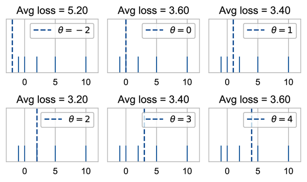
We suggest verifying some of these loss values by hand to check that you understand how the MAE is computed.

Of the values of $\theta$ that we tried, we found that $\theta =2$ has the lowest mean absolute error. For this simple example, 2 is the median of the data values. This isn’t a coincidence. Let’s now check what the average loss is for the original dataset of bus late times. We find the MAE when we set $\theta$ to the mode, median, and mean of the minutes late, respectively:

We see again that the median (middle plot) gives a smaller loss than the mode and mean (left and right plots). In fact, for absolute loss, the minimizing $\hat{\theta }$ is the $\text{median}\{y_1,y_2,\dots ,y_n\}$.

So far, we have found the best value of $\theta$ by simply trying out a few values and then picking the one with the smallest loss. To get a better sense of the MAE as a function of $\theta$, we can try many more values of $\theta$ and plot a curve that shows how $L(\theta ,\mathbf{y})$ changes as $\theta$ changes. We draw the curve for the preceding example with the five data values $[–1,0,2,5,10]$:

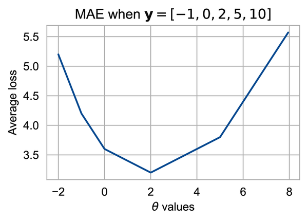
The preceding plot shows that in fact, $\theta =2$ is the best choice for this small dataset of five values. Notice the shape of the curve. It is piecewise linear, where the line segments connect at the location of the data values (–1, 0, 2, and 5). This is a property of the absolute value function. With a lot of data, the flat pieces are less obvious. Our bus data have over 1,400 points and the MAE curve appears smoother:

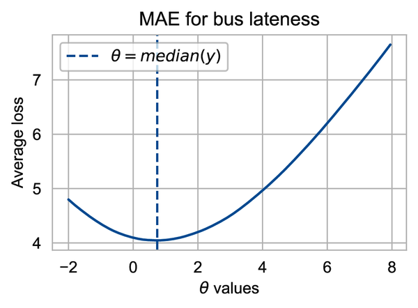
We can use this plot to help confirm that the median of the data is the minimizing value; in other words, $\hat{\theta }=0.74$. This plot is not really a proof, but hopefully it’s convincing enough for you.

Next, let’s look at another loss function that squares error.

Mean Squared Error

We have fitted a constant model to our data and found that with mean absolute error, the minimizer is the median. Now we’ll keep our model the same but switch to a different loss function: squared error. Instead of taking the absolute difference between each data value $y$ and the constant $\theta$, we’ll square the error. That is, for some value of $\theta$ and data value $y$:

1. Find the error, $y-\theta$.

2. Take the square of the error, $(y-\theta {)}^2$.

This gives the loss function $\mathcal{l}(\theta ,y)=(y-\theta {)}^2$.

As before, we want to use all of our data to find the best $\theta$, so we compute the mean squared error, or MSE for short:

$$L(\theta ,\mathbf{y})=L(\theta ,y_1,y_2,\dots ,y_n)=\frac{1}{n}\sum _{i=1}^n(y_i-\theta {)}^2$$

We can write a simple Python function to compute the MSE:

def mse_loss(theta, y_vals):
    return np.mean((y_vals - theta) ** 2)

Let’s again try the mean, median, and mode as potential minimizers of the MSE:

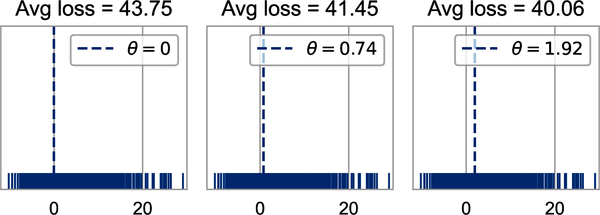
Now when we fit the constant model using MSE loss, we find that the mean (right plot) has a smaller loss than the mode and the median (left and middle plots).

Let’s plot the MSE curve for different values of $\theta$ given our data. The curve shows that the minimizing value $\hat{\theta }$ is close to 2:

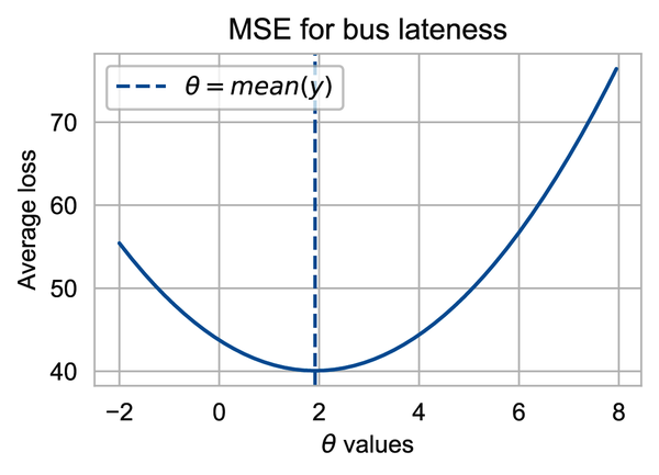
One feature of this curve that is quite noticeable is how rapidly the MSE grows compared to the MAE (note the range on the vertical axis). This growth has to do with the nature of squaring errors; it places a much higher loss on data values further away from $\theta$. If $\theta =10$ and $y=110$, the squared loss is $(10-110{)}^2=10,000$ whereas the absolute loss is $|10-110|=100$. For this reason, the MSE is more sensitive to unusually large data values than the MAE.

From the MSE curve, it appears that the minimizing $\hat{\theta }$ is the mean of $\mathbf{y}$. Again, this is no mere coincidence; the mean of the data always coincides with $\hat{\theta }$ for squared error. We show how this comes about from the quadratic nature of the MSE. Along the way, we demonstrate a common representation of squared loss as a sum of variance and bias terms, which is at the heart of model fitting with squared loss. To begin, we add and subtract $\overline{y}$ in the loss function and expand the square as follows:

$$\begin{array}{r}\begin{array}{rl}L(\theta ,\mathbf{y})& =\frac{1}{n}\sum _{i=1}^n(y_i-\theta {)}^2\\ & =\frac{1}{n}\sum _{i=1}^n[(y_i-\overline{y})+(\overline{y}-\theta ){]}^2\\ & =\frac{1}{n}\sum _{i=1}^n[(y_i-\overline{y}{)}^2+2(y_i-\overline{y})(\overline{y}-\theta )+(\overline{y}-\theta {)}^2]\end{array}\end{array}$$

Next, we split the MSE into the sum of these three terms and note that the middle term is 0, due to the simple property of the average: $\sum (y_i-\overline{y})=0$:

$$\begin{array}{r}\begin{array}{rl}\frac{1}{n}\sum _{i=1}^n& (y_i-\overline{y}{)}^2+\frac{1}{n}\sum _{i=1}^{n}2(y_i-\overline{y})(\overline{y}-\theta )+\frac{1}{n}\sum _{i=1}^n(\overline{y}-\theta {)}^2\\ & =\frac{1}{n}\sum _{i=1}^n(y_i-\overline{y}{)}^2+2(\overline{y}-\theta )\frac{1}{n}\sum _{i=1}^n(y_i-\overline{y})+\frac{1}{n}\sum _{i=1}^n(\overline{y}-\theta {)}^2\\ & =\frac{1}{n}\sum _{i=1}^n(y_i-\overline{y}{)}^2+(\overline{y}-\theta {)}^2\end{array}\end{array}$$

Of the remaining two terms, the first does not involve $\theta$. You probably recognize it as the variance of the data. The second term is always non-negative. It is called the bias squared. This second term, the bias squared, is 0 when $\theta$ is $\overline{y}$, so $\hat{\theta }=\overline{y}$ gives the smallest MSE for any dataset.

We have seen that for absolute loss, the best constant model is the median, but for squared error, it’s the mean. The choice of the loss function is an important aspect of model fitting.

Choosing Loss Functions

Now that we’ve worked with two loss functions, we can return to our original question: how do we choose whether to use the median, mean, or mode? Since these statistics minimize different loss functions,² we can equivalently ask: what is the most appropriate loss function for our problem? To answer this question, we look at the context of our problem.

Compared to the MAE, the MSE gives especially large losses when the bus is much later (or earlier) than expected. A bus rider who wants to understand the typical late times would use the MAE and the median (0.74 minutes late), but a rider who despises unexpected large late times might summarize the data using the MSE and the mean (1.92 minutes late).

If we want to refine the model even more, we can use a more specialized loss function. For example, suppose that when a bus arrives early, it waits at the stop until the scheduled time of departure; then we might want to assign an early arrival 0 loss. And if a really late bus is a larger aggravation than a moderately late one, we might choose an asymmetric loss function that gives a larger penalty to super-late arrivals.

In essence, context matters when choosing a loss function. By thinking carefully about how we plan to use the model, we can pick a loss function that helps us make good data-driven decisions.

Summary

We introduced the constant model: a model that summarizes the data by a single value. To fit the constant model, we chose a loss function that measured how well a given constant fits a data value, and we computed the average loss over all of the data values. We saw that depending on the choice of loss function, we get a different minimizing value: we found that the mean minimizes the average squared error (MSE), and the median minimizes the average absolute error (MAE). We also discussed how we can incorporate context and knowledge of our problem to pick a loss function.

The idea of fitting models through loss minimization ties simple summary statistics—like the mean, median, and mode—to more complex modeling situations. The steps we took to model our data apply to many modeling scenarios:

1. Select the form of a model (such as the constant model).

2. Select a loss function (such as absolute error).

3. Fit the model by minimizing the loss over all the data (such as average loss).

For the rest of this book, our modeling techniques expand upon one or more of these steps. We introduce new models, new loss functions, and new techniques for minimizing loss. Chapter 5 revisits the study of a bus arriving late at its stop. This time, we present the problem as a case study and visit all stages of the data science lifecycle. By going through these stages, we make some unusual discoveries; when we augment our analysis by considering data scope and using an urn to simulate a rider arriving at the bus stop, we find that modeling bus lateness is not the same as modeling the rider’s experience waiting for a bus.

¹ We (the authors) first learned of the bus arrival time data from an analysis by a data scientist named Jake VanderPlas. We’ve named the protagonist of this section in his honor.

² The mode minimizes a loss function called 0-1 loss. Although we haven’t covered this specific loss, the procedure is identical: pick the loss function, then find what minimizes the loss.