Learning Algorithms

Chapter 4. Heaping It On

In this chapter, you will learn:

• The queue and priority queue data types.

• The binary heap data structure, invented in 1964, which can be stored in an array.

• That in a max binary heap, an entry with a larger numeric priority is considered to have higher priority than an entry with a smaller numeric priority. In a min binary heap, entries with smaller numeric priority have higher priority.

• How to enqueue a (value, priority) entry to a binary heap in O(log N), where N is the number of entries in the heap.

• How to find the value with highest priority in a binary heap in O(1).

• How to remove the value with highest priority from a binary heap in O(log N).

Instead of just storing a collection of values, what if you stored a collection of entries, where each entry has a value and an associated priority represented as a number? Given two entries, the one whose priority is higher is more important than the other. The challenge this time is to make it possible to insert new (value, priority) entries into a collection and be able to remove and return the value for the entry with highest priority from the collection.

This behavior defines a priority queue—a data type that efficiently supports enqueue(value, priority) and dequeue(), which removes the value with highest priority. The priority queue is different from the symbol table discussed in the previous chapter because you do not need to know the priority in advance when requesting to remove the value with highest priority.

When a busy nightclub becomes too crowded, a line of people forms outside, as shown in Figure 4-1. As more people try to enter the club, they have to wait at the end of the line. The first person to enter the nightclub from the line is the one who has waited the longest. This behavior represents the essential queue abstract data type, with an enqueue(value) operation that adds value to become the newest value at the end of the queue, and dequeue() removes the oldest value remaining in the queue. Another way to describe this experience is “First in, first out” (FIFO), which is shorthand for “First [one] in [line is the] first [one taken] out [of line].”

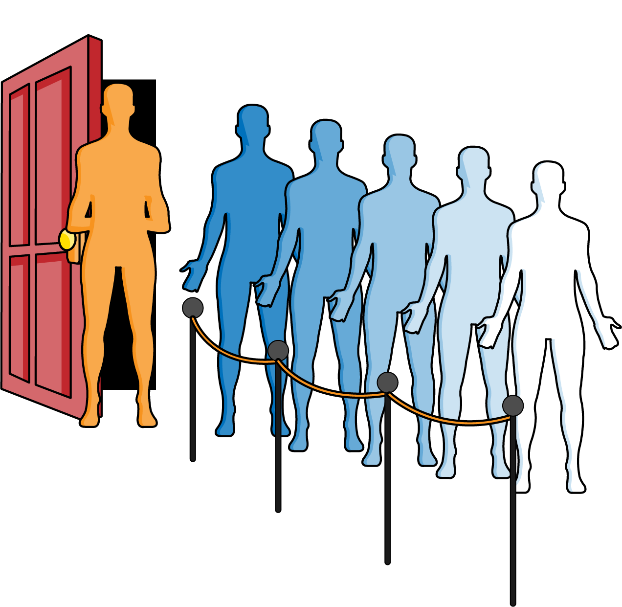
Figure 4-1. Waiting in a queue at a nightclub

In the previous chapter, I described the linked list data structure, which I will use again with a Node that stores a value for the queue:

class Node:
  def __init__(self, val):
    self.value = val
    self.next = None

Using this structure, the Queue implementation in Listing 4-1 has an enqueue() operation to add a value to the end of a linked list. Figure 4-2 shows the result of enqueuing (in this order) “Joe,” “Jane,” and “Jim” to a nightclub queue.

“Joe” will be the first patron dequeued from the line, resulting in a queue with two patrons, where “Jane” remains the first one in line.

In Queue, the enqueue() and dequeue() operations perform in constant time, independent of the total number of values in the queue.

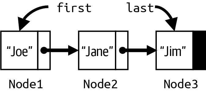
Figure 4-2. Modeling a nightclub queue with three nodes

Listing 4-1. Linked list implementation of Queue data type

class Queue:
  def __init__(self):
    self.first = None                     
    self.last = None

  def is_empty(self):
    return self.first is None             

  def enqueue(self, val):
    if self.first is None:                
      self.first = self.last = Node(val)
    else:
      self.last.next = Node(val)          
      self.last = self.last.next

  def dequeue(self):
    if self.is_empty():
      raise RuntimeError('Queue is empty')

    val = self.first.value                
    self.first = self.first.next          
    return val

Initially, first and last are None.

A Queue is empty if first is None.

If Queue is empty, set first and last to newly created Node.

If Queue is nonempty, add after last, and adjust last to point to newly created Node.

first refers to the Node containing value to be returned.

Set first to be the second Node in the list, should it exist.

Let’s change the situation: the nightclub decides to allow patrons to spend any amount of money to buy a special pass that records the total amount spent. For example, one patron could buy a $50 pass, while another buys a $100 pass. When the club becomes too crowded, people join the line to wait. However, the first person to enter the nightclub from the line is the one holding a pass representing the highest payment of anyone in line. If two or more people in line are tied for having spent the most money, then one of them is chosen to enter the nightclub. Patrons with no pass are treated as having paid $0.

In Figure 4-3, the patron in the middle with a $100 pass is the first one to enter the club, followed by the two $50 patrons (in some order). All other patrons without a pass are considered to be equivalent, and so any one of them could be selected next to enter the club.

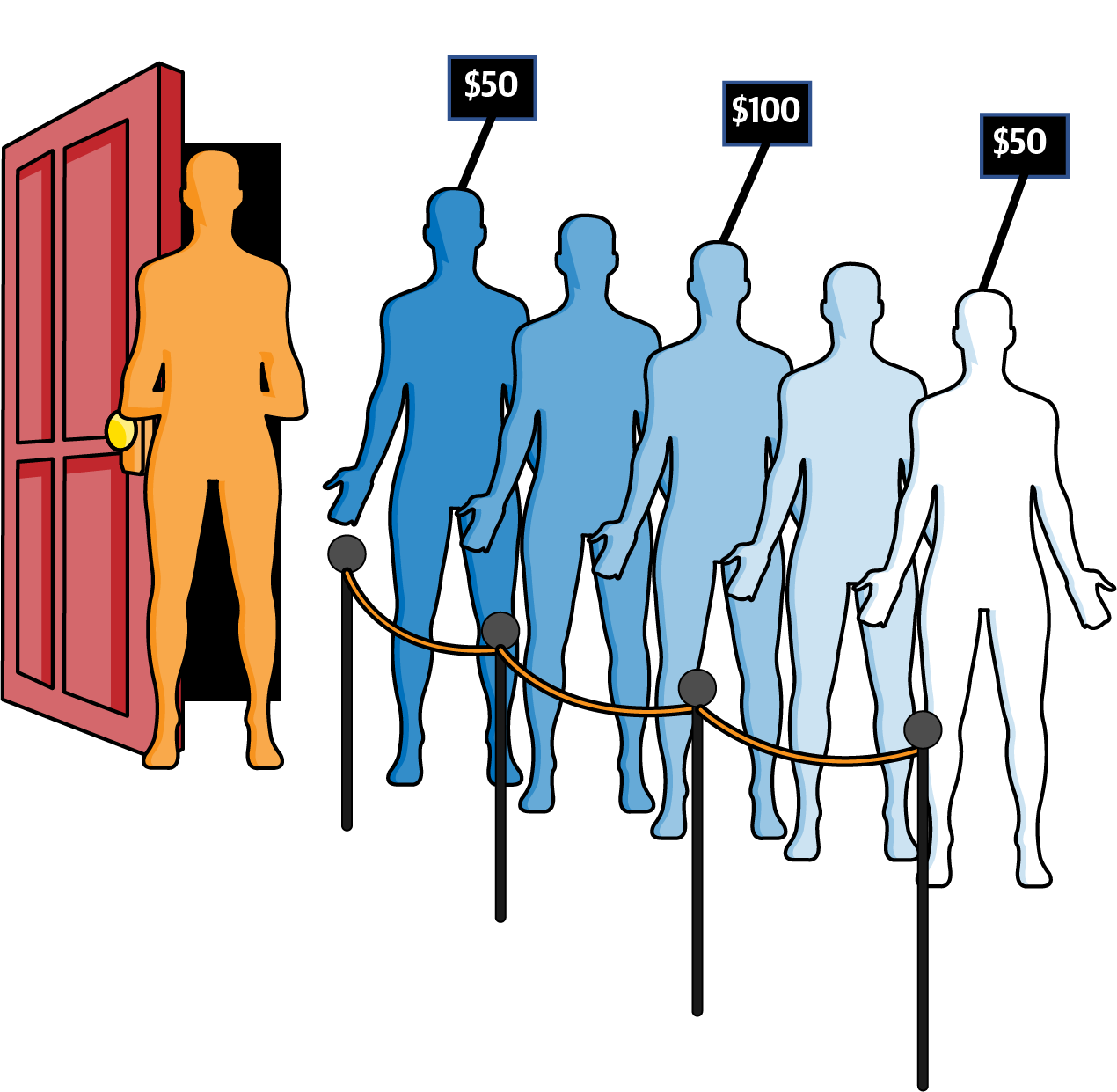
Figure 4-3. Patrons can advance quicker with purchased pass

Note

A priority queue data type does not specify what to do when two or more values share the same highest priority. In fact, based on its implementation, the priority queue might not return values in the order in which they were enqueued. A heap-based priority queue—such as described in this chapter—does not return values with equal priority in the order they were enqueued. The heapq built-in module implements a priority queue using a heap, which I cover in Chapter 8.

This revised behavior defines the priority queue abstract data type; however, enqueue() and dequeue() can no longer be efficiently implemented in constant time. On one hand, if you use a linked list data structure, enqueue() would still be O(1), but dequeue() would potentially have to check all values in the priority queue to locate the one with highest priority, requiring O(N) in the worst case. On the other hand, if you keep all elements in sorted order by priority, dequeue() requires O(1), but now enqueue() requires O(N) in the worst case to find where to insert the new value.

Given our experience to date, here are five possible structures that all use an Entry object to store a (value, priority) entry:

Array

An array of unordered entries that has no structure and hopes for the best. enqueue() is a constant time operation, but dequeue() must search the entire array for the highest priority value to remove and return. Because array has a fixed size, this priority queue could become full.

Built-in

An unordered list manipulated using Python built-in operations that offers similar performance to Array.

OrderA

An array containing entries sorted by increasing priority. On enqueue(), use Binary Array Search variation (from Listing 2-4) to locate where the entry should be placed, and manually shift array entries to make room. dequeue() is constant-time because the entries are fully ordered, and the highest priority entry is found at the end of the array. Because the array has a fixed size, this priority queue could become full.

Linked

A linked list of entries whose first entry has highest priority of all entries in the list; each subsequent entry is smaller than or equal to the previous entry. This implementation enqueues new values into their proper location in the linked list to allow dequeue() to be a constant-time operation.

OrderL

A Python list containing ascending entries by increasing priority. On enqueue(), use Binary Array Search variation to dynamically insert the entry into its proper location. dequeue() is constant time because the highest priority entry is always at the end of the list.

To compare these implementations, I devised an experiment that safely performs 3N/2 enqueue() operations and 3N/2 dequeue() operations. For each implementation, I measure the total execution time and divide by 3N to compute the average operation cost. As shown in Table 4-1, a fixed-size array is the slowest, while built-in Python lists cut the time in half. An array of sorted entries halves the time yet again, and a linked list improves by a further 20%. Even so, the clear winner is OrderL.

Table 4-1. Average operation performance (time in ns) on problem instances of size N

N	Heap	OrderL	Linked	OrderA	Built-in	Array
256	6.4	2.5	3.9	6.0	8.1	13.8
512	7.3	2.8	6.4	9.5	14.9	26.4
1,024	7.9	3.4	12.0	17.8	28.5	52.9
2,048	8.7	4.1	23.2	33.7	57.4	107.7
4,096	9.6	5.3	46.6	65.1	117.5	220.3
8,192	10.1	7.4	95.7	128.4	235.8	446.6
16,384	10.9	11.7	196.4	255.4	470.4	899.9
32,768	11.5	20.3	—	—	—	—
65,536	12.4	36.8	—	—	—	—

For these approaches, the average cost of an enqueue() or dequeue() operation increases in direct proportion to N. The column, labeled “Heap” in Table 4-1, however, shows the performance results using a Heap data structure; its average cost increases in direct proportion to log(N), as you can see from Figure 4-4, and it significantly outperforms the implementation using ordered Python lists. You know you have logarithmic performance when you only see a constant time increase in runtime performance when the problem size doubles. In Table 4-1, with each doubling, the performance time increases by about 0.8 nanoseconds.

The heap data structure, invented in 1964, provides O(log N) performance for the operations of a priority queue. For the rest of this chapter, I am not concerned with the values that are enqueued in an entry—they could be strings or numeric values, or even image data; who cares? I am only concerned with the numeric priority for each entry. In each of the remaining figures in this chapter, only the priorities are shown for the entries that were enqueued. Given two entries in a max heap, the one whose priority is larger in value has higher priority.

A heap has a maximum size, M—known in advance—that can store N < M entries. I now explain the structure of a heap, show how it can grow and shrink over time within its maximum size, and show how an ordinary array stores its N entries.

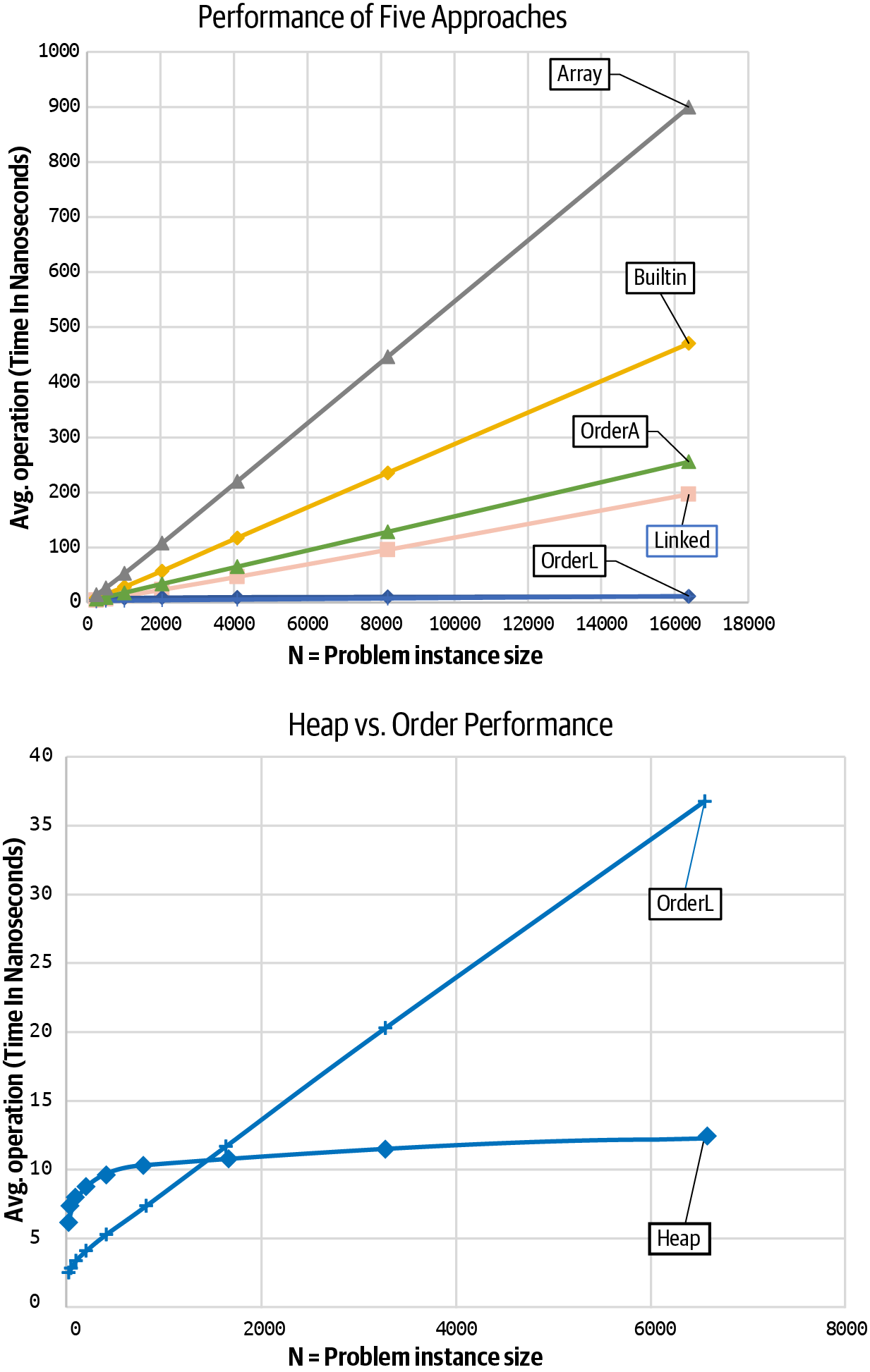
Figure 4-4. O(log N) behavior of Heap outperforms O(N) behavior for other approaches

Max Binary Heaps

It may seem like a strange idea, but what if I only “partially sort” the entries? Figure 4-5 depicts a max heap containing 17 entries; for each entry, only its priority is shown. As you can see, level 0 contains a single entry that has the highest priority among all entries in the max heap. When there is an arrow, x → y, you can see that the priority for entry x ≥ the priority for entry y.

Figure 4-5. A sample max binary heap

These entries are not fully ordered like they would be in a sorted list, so you have to search awhile to find the entry with lowest priority (hint: it’s on level 3). But the resulting structure has some nice properties. There are two entries in level 1, one of which must be the second-highest priority (or tied with the highest one, right?). Each level k—except for the last one—is full and contains 2^k entries. Only the bottommost level is partially filled (i.e., it has 2 entries out of a possible 16), and it is filled from left to right. You can also see that the same priority may exist in the heap—the priorities 8 and 14 appear multiple times.

Each entry has no more than 2 arrows coming out of it, which makes this a max binary heap. Take the entry on level 0 whose priority is 15: the first entry on level 1 with priority 13 is its left child; the second entry on level 1 with priority 14 is its right child. The entry with priority 15 is the parent of the two children entries on level 1.

The following summarizes the properties of a max binary heap:

Heap-ordered property

The priority of an entry is greater than or equal to the priority of its left child and its right child (should either one exist). The priority for each entry (other than the topmost one) is smaller than or equal to the priority of its parent entry.

Heap-shape property

Each level k must be filled with 2^k entries (from left to right) before any entry appears on level k + 1.

When a binary heap only contains a single entry, there is just a single level, 0, because 2⁰ = 1. How many levels are needed for a binary heap to store N > 0 entries? Mathematically, I need to define a formula, L(N), that returns the number of necessary levels for N entries. Figure 4-6 contains a visualization to help determine L(N). It contains 16 entries, each labeled using a subscript that starts at e₁ at the top and increases from left to right until there are no more entries on that level, before starting again at the leftmost entry on the next level.

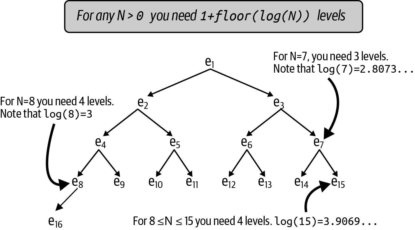
Figure 4-6. Determining levels needed for a binary heap with N entries

If there were only 7 entries in a heap, there would be 3 levels containing entries e₁ through e₇. Four levels would be needed for 8 entries. If you follow the left arrows from the top, you can see that the subscripts follow a specific pattern: e₁, e₂, e₄, e₈, and e₁₆, suggesting that powers of 2 will play a role. It turns out that L(N) = 1 + floor(log(N)).

Tip

Each new full level in the binary heap contains more entries than the total number of entries in all previous levels. When you increase the height of a binary heap by just one level, the binary heap can contain more than twice as many entries (a total of 2N + 1 entries, where N is the number of existing entries)!

You should recall with logarithms that when you double N, the value of log(N) increases by 1. This is represented mathematically as follows: log(2N) = 1 + log(N). Which of the four options in Figure 4-7 are valid max binary heaps?

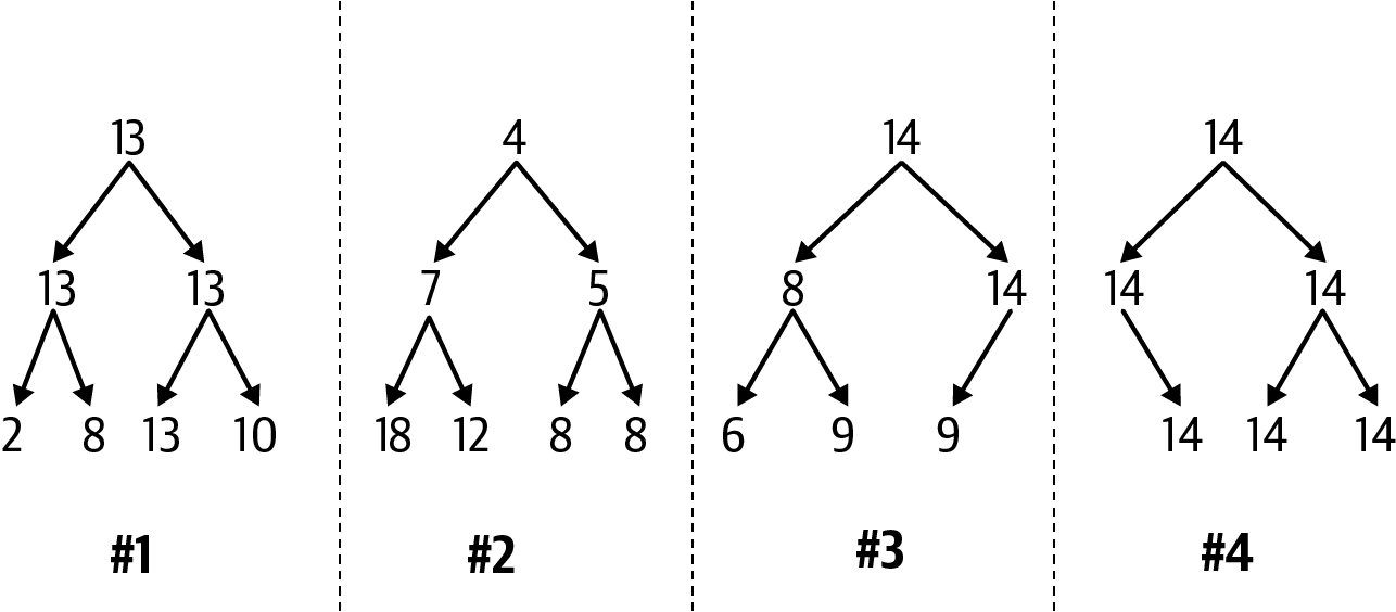
Figure 4-7. Which of these are valid max binary heaps?

First review the heap-shape property for each of these options. Options #1 and #2 are acceptable, since each level is completely full. Option #3 is acceptable because only its last level is partial and it contains three (out of possible four) entries from left to right. Option #4 violates the heap-shape property because its last level contains three entries, but the leftmost possible entry is missing.

Now consider the heap-ordered property for max binary heaps, which ensures that each parent’s priority is greater than or equal to the priorities of its children. Option #1 is valid, as you can confirm by checking each possible arrow. Option #3 is invalid because the entry with priority 8 has a right child whose priority of 9 is greater. Option #2 is invalid because the entry with priority 4 on level 0 has smaller priority than both of its children entries.

Note

Option #2 is actually a valid example of a min binary heap, where each parent entry’s priority is smaller than or equal to the priority of its children. Min binary heaps will be used in Chapter 7.

I need to make sure that both heap properties hold after enqueue() or dequeue() (which removes the value with highest priority in the max heap). This is important because then I can demonstrate that both of these operations will perform in O(log N), a significant improvement to the approaches documented earlier in Table 4-1, which were limited since either enqueue() or dequeue() had worst case behavior of O(N).

Inserting a (value, priority)

After enqueue(value, priority) is invoked on a max binary heap, where should the new entry be placed? Here’s a strategy that always works:

• Place the new entry into the first available empty location on the last level.

• If that level is full, then extend the heap to add a new level, and place the new entry in the leftmost location in the new level.

In Figure 4-8, a new entry with priority 12 is inserted in the third location on level 4. You can confirm that the heap-shape property is valid (because the entries on the partial level 4 start from the left with no gaps). It might be the case, however, that the heap-ordered property has now been violated.

The good news is that I only need to possibly rearrange entries that lie in the path from the newly placed entry all the way back to the topmost entry on level 0. Figure 4-10 shows the end result after restoring the heap-ordered property; as you can see, the entries in the shaded path have been reordered appropriately, in decreasing (or equal) order from the top downward.

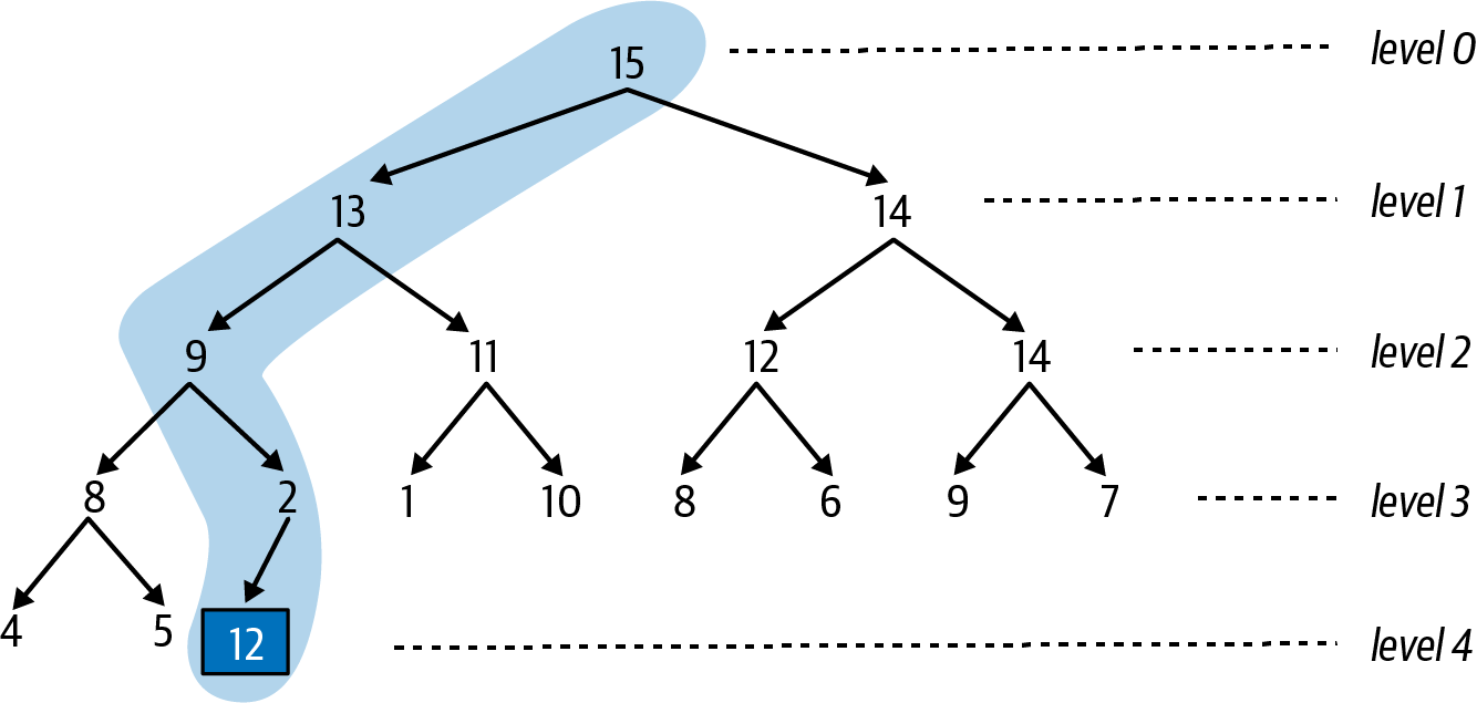
Figure 4-8. The first step in inserting an entry is placing it in the next available position

Note

A path to a specific entry in a binary heap is a sequence of entries formed by following the arrows (left or right) from the single entry on level 0 until you reach the specific entry.

To remake the max heap to satisfy the heap-ordered property, the newly added entry “swims up” along this path to its proper location, using pairwise swaps. Based on this example, Figure 4-8 shows that the newly added entry with priority 12 invalidates the heap-ordered priority since its priority is larger than its parent whose priority is 2. Swap these two entries to produce the max heap in Figure 4-9 and continue upward.

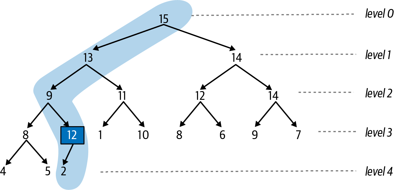
Figure 4-9. The second step swims the entry up one level as needed

You can confirm that from 12 downward, the structure is a valid max binary heap with two entries. However the entry with 12 still invalidates the heap-ordered property since its parent entry has a priority of 9, which is smaller, so swap with its parent, as shown in Figure 4-10.

From highlighted entry 12 downward in Figure 4-10, the structure is a valid max binary heap. When you swapped the 9 and 12 entries, you didn’t have to worry about the structure from 8 and below since all of those values are known to be smaller than or equal to 8, which means they will all be smaller than or equal to 12. Since 12 is smaller than its parent entry with priority of 13, the heap-ordered property is satisfied.

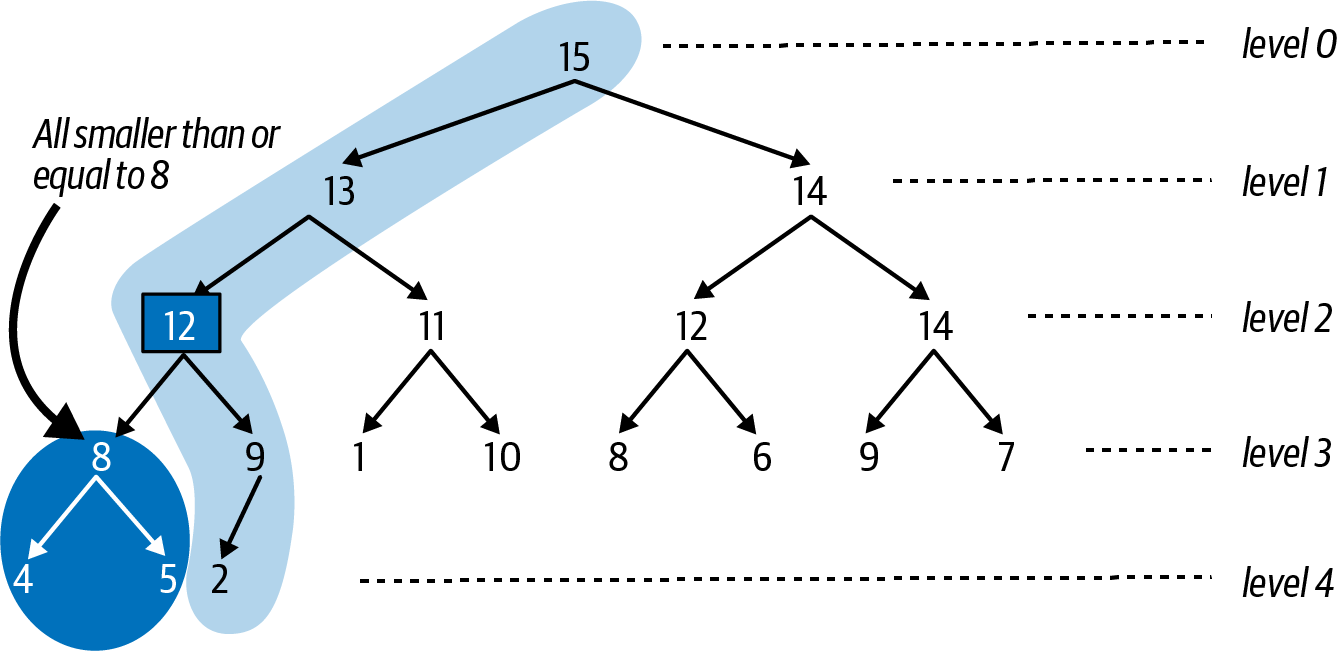
Figure 4-10. Third step swims the entry up one level as needed

Try on your own to enqueue(value, 16) into the heap depicted in Figure 4-10, which initially places the new entry in the fourth location on level 4, as the right child of the entry with priority 9. This new entry will swim up all the way to level 0, resulting in the max binary heap shown in Figure 4-11.

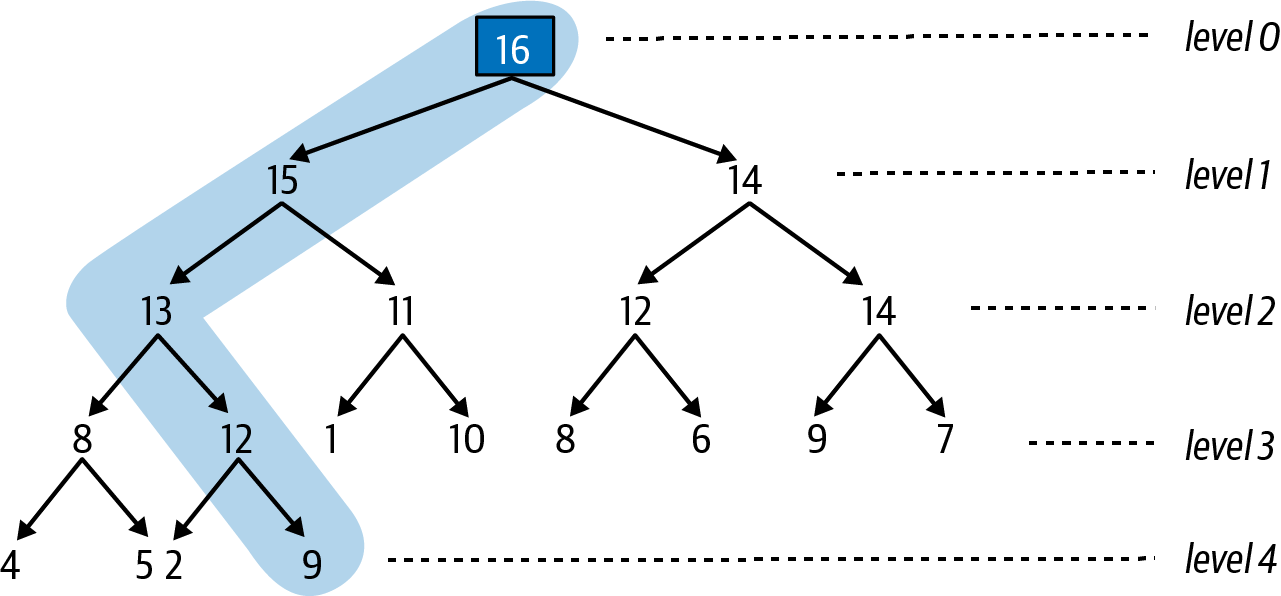
Figure 4-11. Adding entry with priority 16 swims up to the top

The worst case is when you enqueue a new entry whose priority is higher than any entry in the max binary heap. The number of entries in the path is 1 + floor(log(N)), which means the most number of swaps is one smaller, or floor(log(N)). Now I can state clearly that the time to remake the max binary heap after an enqueue() operation is O(log N). This great result only addresses half of the problem, since I must also ensure that I can efficiently remove the entry with highest priority in the max binary heap.

Removing the Value with Highest Priority

Finding the entry with highest priority in a max binary heap is simple—it will always be the single entry on level 0 at the top. But you just can’t remove that entry, since then the heap-shape property would be violated by having a gap at level 0. Fortunately, there is a dequeue() strategy that can remove the topmost entry and efficiently remake the max binary heap, as I show in the next sequence of figures:

1. Remove the rightmost entry on the bottommost level and remember it. The resulting structure will satisfy both the heap-ordered and heap-shape properties.

2. Save the value for the highest priority entry on level 0 so it can be returned.

3. Replace the entry on level 0 with the entry you removed from the bottommost level of the heap. This might break the heap-ordered property.

To achieve this goal, first remove and remember entry 9, as shown in Figure 4-12; the resulting structure remains a heap. Next, record the value associated with the highest priority on level 0 so it can be returned (not shown here).

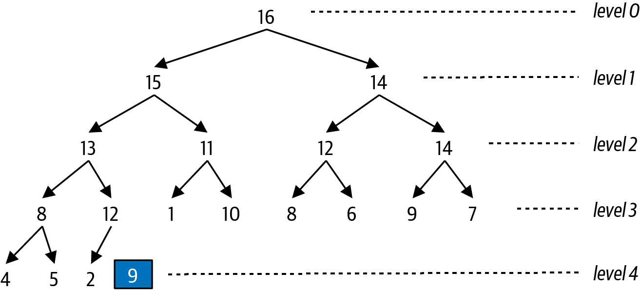
Figure 4-12. First step is to remove bottommost entry

Finally, replace the single entry on level 0 with the entry that was removed, resulting in the broken max heap shown in Figure 4-13. As you can see, the priority of the single entry on level 0 is not greater than its left child (with priority 15) and right child (with priority 14). To remake the max heap, you need to “sink down” this entry to a location further down inside the heap to re-establish the heap-ordered property.

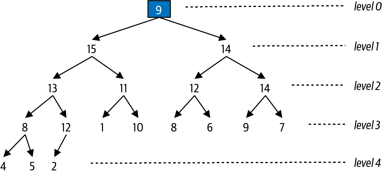
Figure 4-13. Broken heap resulting from swapping last entry with level 0

Starting from the entry that is invalid (i.e., the level 0 entry with priority 9), determine which of its children (i.e., left or right) has the higher priority—if only the left child exists, then use that one. In this running example, the left child with priority 15 has higher priority than the right child with priority 14, and Figure 4-14 shows the result of swapping the topmost entry with the higher selected child entry.

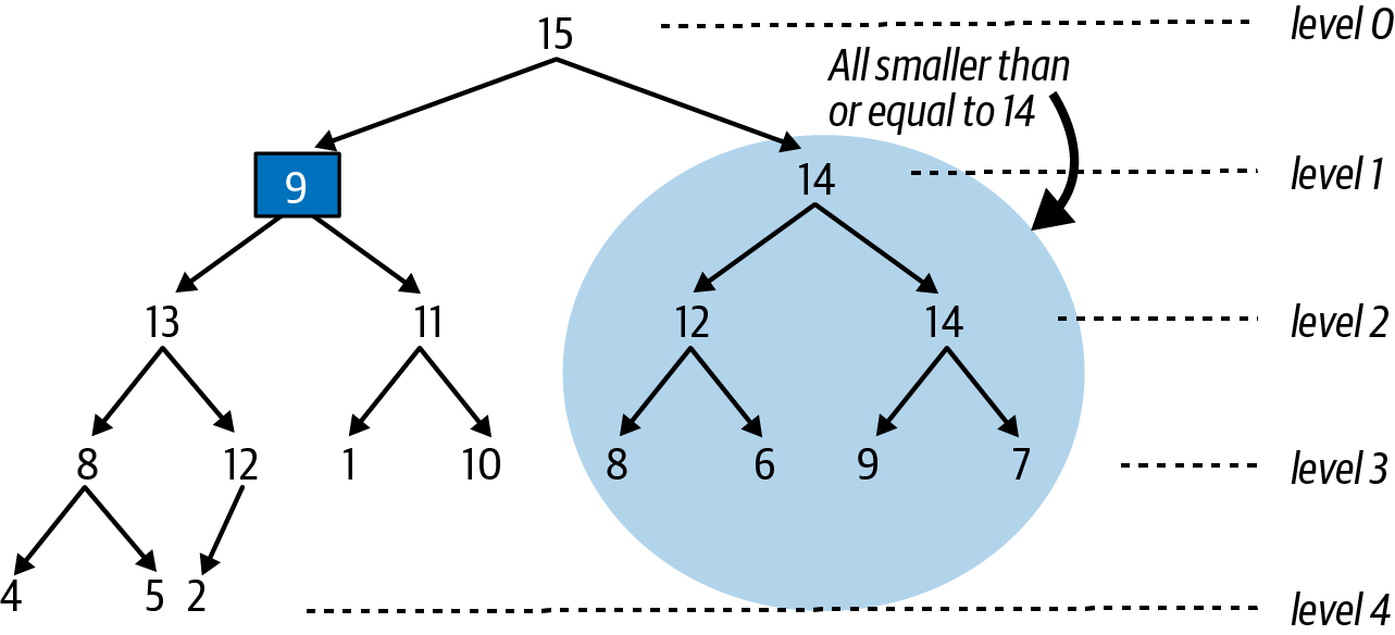
Figure 4-14. Swapping the top entry with its left child, which had higher priority

As you can see, the entire substructure based on the entry with priority 14 on level 1 is a valid max binary heap, and so it doesn’t need to change. However, the newly swapped entry (with priority 9) violates the heap-ordered property (it is smaller than the priority of both of its children), so this entry must continue to “sink down” to the left, as shown in Figure 4-15, since the entry with priority 13 is the larger of its two children entries.

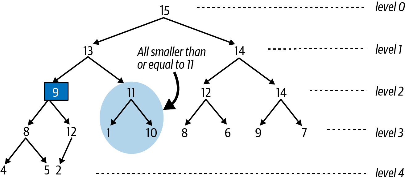
Figure 4-15. Sinking down one an additional level

Almost there! Figure 4-15 shows that the entry with priority 9 has a right child whose priority of 12 is higher, so we swap these entries, which finally restores the heap-ordered property for this heap, as shown in Figure 4-16.

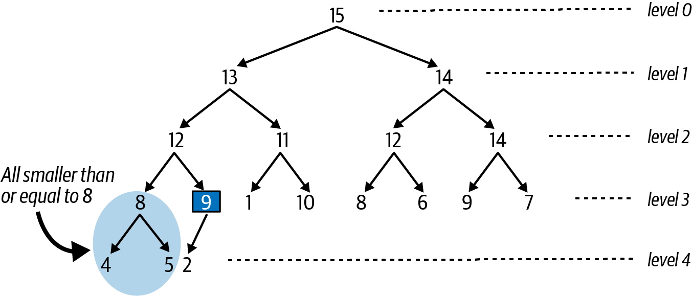
Figure 4-16. Resulting heap after sinking entry to its proper location

There is no simple path of adjusted entries, as we saw when enqueuing a new entry to the priority queue, but it is still possible to determine the maximum number of times the “sink down” step was repeated, namely, one value smaller than the number of levels in the max binary heap, or floor(log(N)).

You can also count the number of times the priorities of two entries were compared with each other. For each “sink down” step, there are at most two comparisons—one comparison to find the larger of the two sibling entries, and then one comparison to determine if the parent is bigger than the larger of these two siblings. In total, this means the number of comparisons is no greater than 2 × floor(log(N)).

It is incredibly important that the max binary heap can both add an entry and remove the entry with highest priority in time that is directly proportional to log(N) in the worst case. Now it is time to put this theory into practice by showing how to implement a binary heap using an ordinary array.

Have you noticed that the heap-shape property ensures that you can read all entries in sequence from left to right, from level 0 down through each subsequent level? I can take advantage of this insight by storing a binary heap in an ordinary array.

Representing a Binary Heap in an Array

Figure 4-17 shows how to store a max binary heap of N = 18 entries within a fixed array of size M > N. This max binary heap of five levels can be stored in an ordinary array by mapping each location in the binary heap to a unique index location. Each dashed box contains an integer that corresponds to the index position in the array that stores the entry from the binary heap. Once again, when depicting a binary heap, I only show the priorities of the entries.

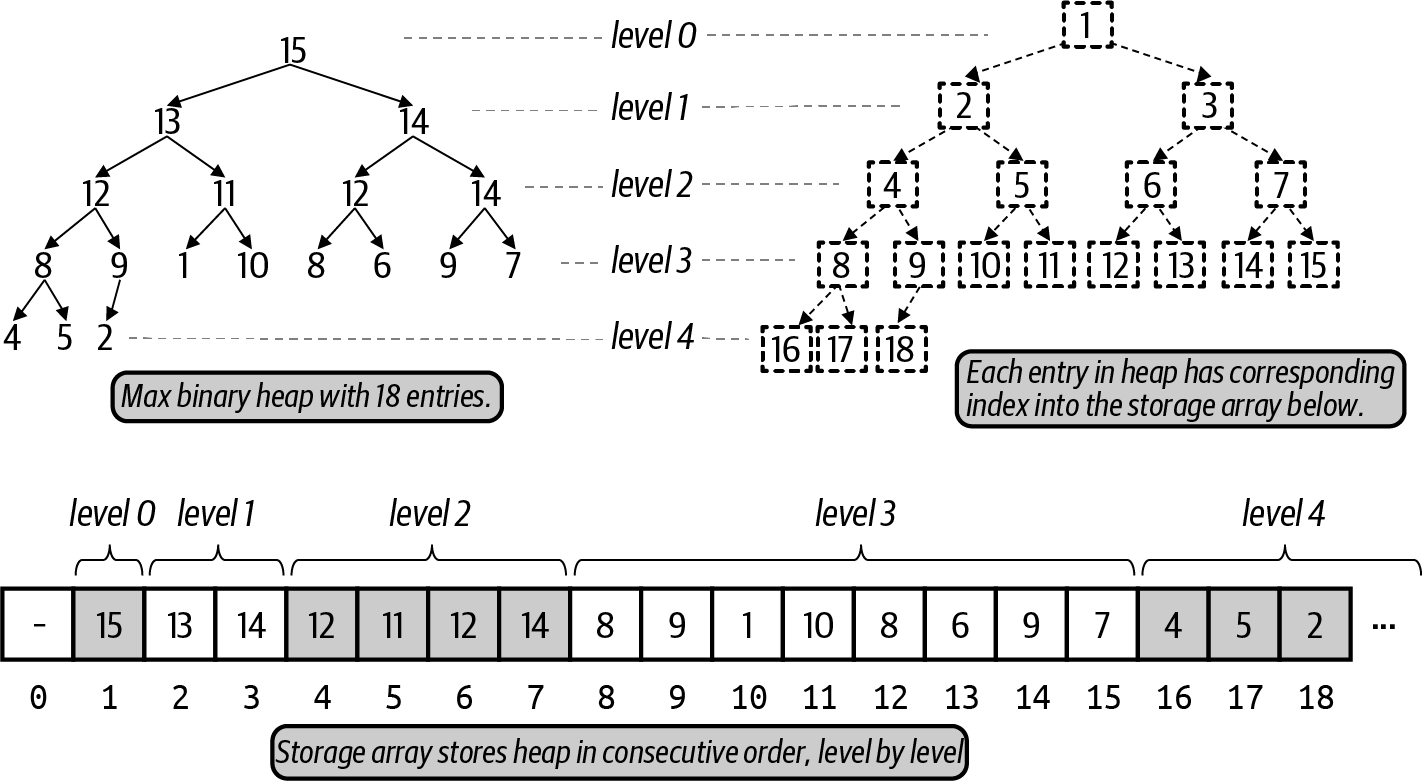
Figure 4-17. Storing a max binary heap in an array

Each entry has a corresponding location in the storage[] array. To simplify all computations, location storage[0] is unused and never stores an entry. The topmost entry with priority 15 is placed in storage[1]. You can see that its left child, with priority 13, is placed in storage[2]. If the entry in storage[k] has a left child, that entry is storage[2*k]; Figure 4-17 confirms this observation (just inspect the dashed boxes). Similarly, if the entry in storage[k] has a right child, that entry is in storage[2*k+1].

For k > 1, the parent of the entry in storage[k] can be found in storage[k//2], where k//2 is the integer value resulting by truncating the result of k divided by 2. By placing the topmost entry of the heap in storage[1], you just perform integer division by two to compute the parent location of an entry. The parent of the entry in storage[5] (with a priority of 11) is found in storage[2] because 5//2 = 2.

The entry in storage[k] is a valid entry when 0 < k ≤ N, where N represents the number of entries in the max binary heap. This means that the entry at storage[k] has no children if 2 × k > N; for example, the entry at storage[10] (which has priority of 1) has no left child, because 2 × 10 = 20 > 18. You also know that the entry at storage[9] (which coincidentally has a priority of 9) has no right child, because 2 × 9 + 1 = 19 > 18.

Implementation of Swim and Sink

To store a max binary heap, start with an Entry that has a value with its associated priority:

class Entry:
  def __init__(self, v, p):
    self.value = v
    self.priority = p

Listing 4-2 stores a max binary heap in an array, storage. When instantiated, the length of storage is one greater than the size parameter, to conform to the computations described earlier where the first entry is stored in storage[1].

There are two helper methods that simplify the presentation of the code. You have seen how many times I checked whether one entry has a smaller priority than another entry. The less(i,j) function returns True when the priority of the entry in storage[i] is smaller than the priority of the entry in storage[j]. When swimming up or sinking down, I need to swap two entries. The swap(i,j) function swaps the locations of the entries in storage[i] and storage[j].

Listing 4-2. Heap implementation showing enqueue() and swim() methods

class PQ:
  def less(self, i, j):                               
    return self.storage[i].priority < self.storage[j].priority

  def swap(self, i, j):                               
    self.storage[i],self.storage[j] = self.storage[j],self.storage[i]

  def __init__(self, size):                           
    self.size = size
    self.storage = [None] * (size+1)
    self.N = 0

  def enqueue(self, v, p):                            
    if self.N == self.size:
      raise RuntimeError ('Priority Queue is Full!')

    self.N += 1
    self.storage[self.N] = Entry(v, p)
    self.swim(self.N)

  def swim(self, child):                              
    while child > 1 and self.less(child//2, child):   
      self.swap(child, child//2)                      
      child = child // 2                              

less() determines if storage[i] has lower priority than storage[j].

swap() switches the locations of entries i and j.

storage[1] through storage[size] will store the entries; storage[0] is unused.

To enqueue a (v, p) entry, place it in the next empty location and swim it upward.

swim() remakes the storage array to conform to the heap-ordered property.

The parent of the entry in storage[child] is found in storage[child//2], where child//2 is the integer result of dividing child by 2.

Swap entries at storage[child] and its parent storage[child//2].

Continue upward by setting child to its parent location as needed.

The swim() method is truly brief! The entry identified by child is the newly enqueued entry, while child//2 is its parent entry, should it exist. If the parent entry has lower priority than the child, they are swapped, and the process continues upward.

Figure 4-18 shows the changes to storage initiated by enqueue(value, 12) in Figure 4-8. Each subsequent row corresponds to an earlier identified figure and shows the entries that change in storage. The final row represents a max binary heap that conforms to the heap-ordered and heap-shape properties.

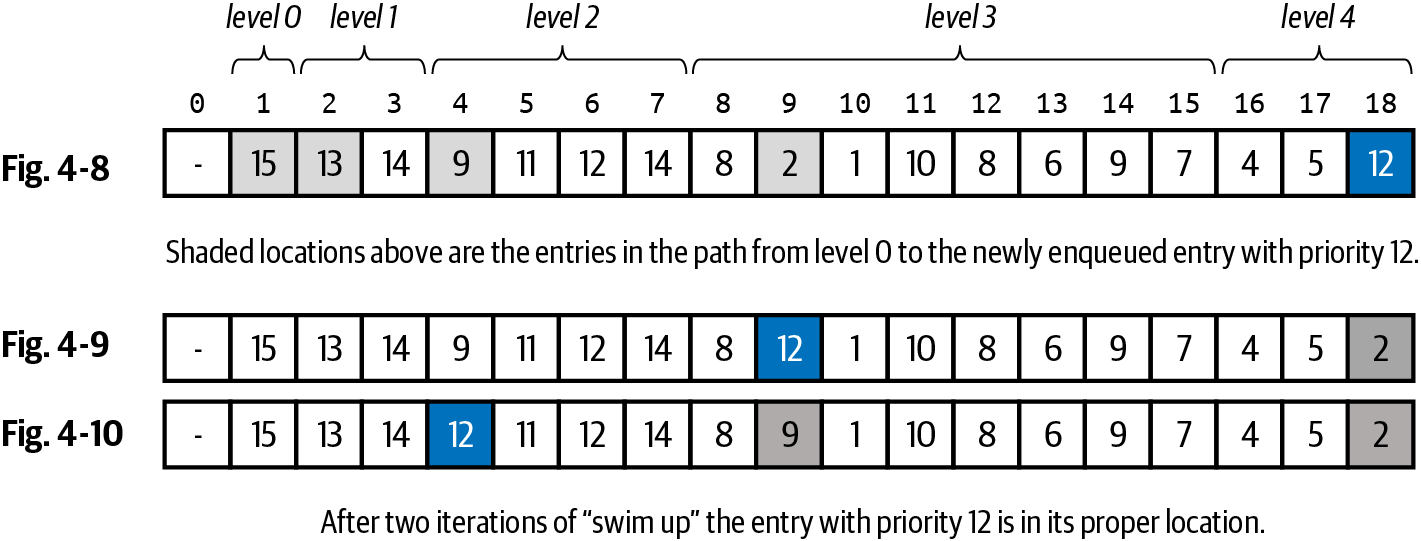
Figure 4-18. Changes to storage after enqueue in Figure 4-8

The path from the topmost entry to the newly inserted entry with priority 12 consists of five entries, as shaded in Figure 4-18. After two times through the while loop in swim(), the entry with priority 12 is swapped with its parent, eventually swimming up to storage[4], where it satisfies the heap-ordered property. The number of swaps will never be more than log(N), where N is the number of entries in the binary heap.

The implementation in Listing 4-3 contains the sink() method to reestablish the structure of the max binary heap after dequeue() is invoked.

Listing 4-3. Heap implementation completed with dequeue() and sink() methods

  def dequeue(self):
    if self.N == 0:
      raise RuntimeError ('PriorityQueue is empty!')

    max_entry = self.storage[1]                         
    self.storage[1] = self.storage[self.N]              
    self.storage[self.N] = None
    self.N -= 1                                         
    self.sink(1)
    return max_entry.value                              

  def sink(self, parent):
    while 2*parent <= self.N:                           
      child = 2*parent
      if child < self.N and self.less(child, child+1):  
        child += 1
      if not self.less(parent, child)                   
        break
      self.swap(child, parent)                          
      parent = child

Save entry of highest priority on level 0.

Replace entry in storage[1] with entry from bottommost level of heap and clear from storage.

Reduce number of entries before invoking sink on storage[1].

Return the value associated with entry of highest priority.

Continue checking as long as parent has a child.

Select right child if it exists and is larger than left child.

If parent is not smaller than child, heap-ordered property is met.

Swap if needed, and continue sinking down, using child as new parent.

Figure 4-19 shows the changes to storage initiated by dequeue() based on the initial max binary heap shown in Figure 4-11. The first row of Figure 4-19 shows the array with 19 entries. In the second row, the final entry in the heap with priority 9 is swapped to become the topmost entry in the max binary heap, which breaks the heap-ordered property; also, the heap now only contains 18 entries, since one was deleted.

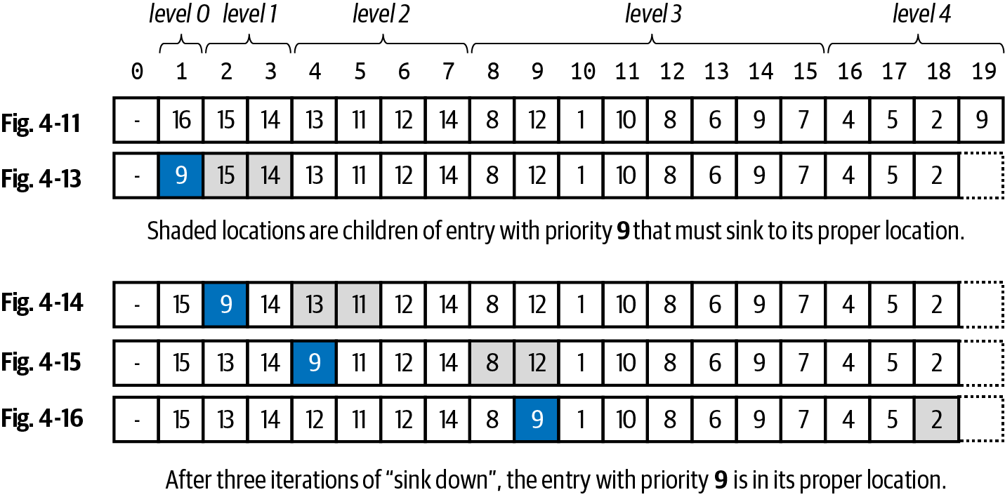
Figure 4-19. Changes to storage after dequeue in Figure 4-11

After three successive passes through the while loop in sink(), the entry with priority 9 has dropped down to a location that ensures the heap-ordered property. In each row, the leftmost highlighted entry is the entry with priority 9, and the shaded entries to the right are its children entries. Whenever the parent entry of 9 is smaller than one of its children, it must sink down to be swapped with the larger of its children. The number of swaps will never be more than log(N).

The sink() method is the hardest to visualize because there is no straight path to follow, as with swim(). In the final representation of storage in Figure 4-19, you can see that the highlighted entry with priority 9 only has one shaded child (with priority 2). When sink() terminates, you know that the entry that was sinking has either reached an index location, p, where it has no children (i.e., because 2 × p is an invalid storage index location greater than N), or it is greater than or equal (i.e., not lesser than) the larger of its children entries.

Warning

The order of the statements in dequeue() is critical. In particular, you have to reduce N by 1 before calling sink(1), otherwise sink() will mistakenly think the index location in storage corresponding to the recently dequeued entry is still part of the heap. You can see in the code that storage[N] is set to None to ensure that entry is not mistakenly thought to be part of the heap.

If you want to convince yourself that the dequeue() logic is correct, consider how it operates with a heap that contains just a single entry. It will retrieve max_entry and set N to 0 before calling sink(), which will do nothing since 2 × 1 > 0.

Summary

The binary heap structure offers an efficient implementation of the priority queue abstract data type. Numerous algorithms, such as those discussed in Chapter 7, depend on priority queues.

• You can enqueue() a (value, priority) entry in O(log N) performance.

• You can dequeue() the entry with highest priority in O(log N) performance.

• You can report the number of entries in a heap in O(1) performance.

In this chapter I focused exclusively on max binary heaps. You only need to make one small change to realize a min binary heap, where higher priority entries have smaller numeric priority values. This will become relevant in Chapter 7. In Listing 4-2, just rewrite the less() method to use greater-than (>) instead of less-than (<). All other code remains the same.

def less(self, i, j):
  return self.storage[i].priority > self.storage[j].priority

While a priority queue can grow or shrink over time, the heap-based implementation predetermines an initial size, M, to store the N < M entries. Once the heap is full, no more additional entries can be enqueued to the priority queue. It is possible to automatically grow (and shrink) the storage array, similar to what I showed in Chapter 3. As long as you use geometric resizing, which doubles the size of storage when it is full, then the overall amortized performance for enqueue() remains O(log N).

Challenge Exercises

1. It is possible to use a fixed array, storage, as the data structure to efficiently implement a queue, such that the enqueue() and dequeue() operations have O(1) performance. This approach is known as a circular queue, which makes the novel suggestion that the first value in the array isn’t always storage[0]. Instead, keep track of first, the index position for the oldest value in the queue, and last, the index position where the next enqueued value will be placed, as shown in Figure 4-20.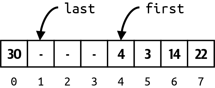

   

   Figure 4-20. Using an array as a circular queue

   As you enqueue and dequeue values, you need to carefully manipulate these values. You will find it useful to keep track of N, the number of values already in the queue. Can you complete the implementation in Listing 4-4 and validate that these operations complete in constant time? You should expect to use the modulo % operator in your code.

   Listing 4-4. Complete this Queue implementation of a circular queue

   class Queue:
     def __init__(self, size):
       self.size = size
       self.storage = [None] * size
       self.first = 0
       self.last = 0
       self.N = 0
   
     def is_empty(self):
       return self.N == 0
   
     def is_full(self):
       return self.N == self.size
   
     def enqueue(self, item):
       """If not full, enqueue item in O(1) performance."""
   
     def dequeue(self):
       """If not empty, dequeue head in O(1) performance."""

2. Insert N = 2^k – 1 elements in ascending order into an empty max binary heap of size N. When you inspect the underlying array that results (aside from the index location 0, which is unused), can you predict the index locations for the largest k values in the storage array? If you insert N elements in descending order into an empty max heap, can you predict the index locations for all N values?

3. Given two max heaps of size M and N, devise an algorithm that returns an array of size M + N containing the combined items from M and N in ascending order in O(M log M + N log N) performance. Generate a table of runtime performance to provide empirical evidence that your algorithm is working.

4. Use a max binary heap to find the k smallest values from a collection of N elements in O(N log k). Generate a table of runtime performance to provide empirical evidence that your algorithm is working.

5. In a max binary heap, each parent entry has up to two children. Consider an alternative strategy, which I call a factorial heap, where the top entry has two children; each of these children has three children (which I’ll call grandchildren). Each of these grandchildren has four children, and so on, as shown in Figure 4-21. In each successive level, entries have one additional child. The heap-shape and heap-ordered property remain in effect. Complete the implementation by storing the factorial heap in an array, and perform empirical evaluation to confirm that the results are slower than max binary heap. Classifying the runtime performance is more complicated, but you should be able to determine that it is O(log N/log(log N)).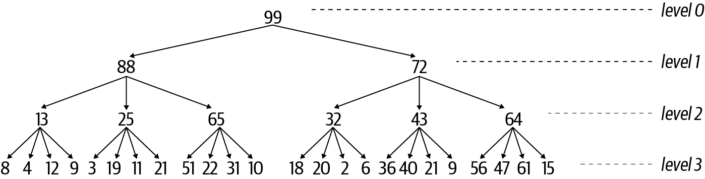

   

   Figure 4-21. A novel factorial heap structure

6. Using the geometric resizing strategy from Chapter 3, extend the PQ implementation in this chapter to automatically resize the storage array by doubling in size when full and shrinking in half when ¼ full.

7. An iterator for an array-based heap data structure should produce the values in the order they would be dequeued without modifying the underlying array (since an iterator should have no side effect). However, this cannot be accomplished easily, since dequeuing values would actually modify the structure of the heap. One solution is to create an iterator(pq) generator function that takes in a priority queue, pq, and creates a separate pqit priority queue whose values are index locations in the storage array for pq, and whose priorities are equal to the corresponding priorities for these values. pqit directly accesses the array storage for pq to keep track of the entries to be returned without disturbing the contents of storage.

   Complete the following implementation, which starts by inserting into pqit the index position, 1, which refers to the pair in pq with highest priority. Complete the rest of the while loop:

   def iterator(pq):
     pqit = PQ(len(pq))
     pqit.enqueue(1, pq.storage[1].priority)
   
     while pqit:
       idx = pqit.dequeue()
       yield (pq.storage[idx].value, pq.storage[idx].priority)
   
       ...

   As long as the original pq remains unchanged, this iterator will yield each of the values in priority order.

Interactive Practice

Get more hands-on training and test your understanding of the concepts by working through our playlist of interactive scenarios. Each step of the scenario must be completed correctly before you can move to the next step. If you get stuck, you can view the solution and learn how to complete the step.

The following scenarios cover material from this chapter:

• Binary Heap Structure: Visualizing Binary Heaps

• Binary Heap Structure: Implementing Binary Heaps

• Binary Heap Structure: Finding k Smallest Values in an Unordered List of N Values