Chapter 4. Linear Algebra
Is there anything more useless or less useful than algebra?
Billy Connolly
Linear algebra is the branch of mathematics that deals with vector spaces. Although I can’t hope to teach you linear algebra in a brief chapter, it underpins a large number of data science concepts and techniques, which means I owe it to you to at least try. What we learn in this chapter we’ll use heavily throughout the rest of the book.
Vectors
Abstractly, vectors are objects that can be added together to form new vectors and that can be multiplied by scalars (i.e., numbers), also to form new vectors.
Concretely (for us), vectors are points in some finite-dimensional space. Although you might not think of your data as vectors, they are often a useful way to represent numeric data.
For example, if you have the heights, weights, and ages of a large number of people, you can treat your data as three-dimensional vectors [height, weight, age]. If you’re teaching a class with four exams, you can treat student grades as four-dimensional vectors [exam1, exam2, exam3, exam4].
The simplest from-scratch approach is to represent vectors as lists of numbers. A list of three numbers corresponds to a vector in three-dimensional space, and vice versa.
We’ll accomplish this with a type alias that says a Vector is just a list of floats:
fromtypingimportListVector=List[float]height_weight_age=[70,# inches,170,# pounds,40]# yearsgrades=[95,# exam180,# exam275,# exam362]# exam4
We’ll also want to perform arithmetic on vectors. Because Python lists aren’t vectors (and hence provide no facilities for vector arithmetic), we’ll need to build these arithmetic tools ourselves. So let’s start with that.
To begin with, we’ll frequently need to add two vectors. Vectors add componentwise. This means that if two vectors v and w are the same length, their sum is just the vector whose first element is v[0] + w[0], whose second element is v[1] + w[1], and so on. (If they’re not the same length, then we’re not allowed to add them.)
For example, adding the vectors [1, 2] and [2, 1] results in [1 + 2, 2 + 1] or [3, 3], as shown in Figure 4-1.
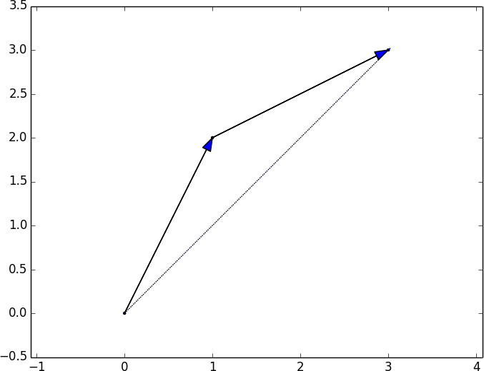
Figure 4-1. Adding two vectors
We can easily implement this by zip-ing the vectors together and using a list comprehension to add the corresponding elements:
defadd(v:Vector,w:Vector)->Vector:"""Adds corresponding elements"""assertlen(v)==len(w),"vectors must be the same length"return[v_i+w_iforv_i,w_iinzip(v,w)]assertadd([1,2,3],[4,5,6])==[5,7,9]
Similarly, to subtract two vectors we just subtract the corresponding elements:
defsubtract(v:Vector,w:Vector)->Vector:"""Subtracts corresponding elements"""assertlen(v)==len(w),"vectors must be the same length"return[v_i-w_iforv_i,w_iinzip(v,w)]assertsubtract([5,7,9],[4,5,6])==[1,2,3]
We’ll also sometimes want to componentwise sum a list of vectors—that is, create a new vector whose first element is the sum of all the first elements, whose second element is the sum of all the second elements, and so on:
defvector_sum(vectors:List[Vector])->Vector:"""Sums all corresponding elements"""# Check that vectors is not emptyassertvectors,"no vectors provided!"# Check the vectors are all the same sizenum_elements=len(vectors[0])assertall(len(v)==num_elementsforvinvectors),"different sizes!"# the i-th element of the result is the sum of every vector[i]return[sum(vector[i]forvectorinvectors)foriinrange(num_elements)]assertvector_sum([[1,2],[3,4],[5,6],[7,8]])==[16,20]
We’ll also need to be able to multiply a vector by a scalar, which we do simply by multiplying each element of the vector by that number:
defscalar_multiply(c:float,v:Vector)->Vector:"""Multiplies every element by c"""return[c*v_iforv_iinv]assertscalar_multiply(2,[1,2,3])==[2,4,6]
This allows us to compute the componentwise means of a list of (same-sized) vectors:
defvector_mean(vectors:List[Vector])->Vector:"""Computes the element-wise average"""n=len(vectors)returnscalar_multiply(1/n,vector_sum(vectors))assertvector_mean([[1,2],[3,4],[5,6]])==[3,4]
A less obvious tool is the dot product. The dot product of two vectors is the sum of their componentwise products:
defdot(v:Vector,w:Vector)->float:"""Computes v_1 * w_1 + ... + v_n * w_n"""assertlen(v)==len(w),"vectors must be same length"returnsum(v_i*w_iforv_i,w_iinzip(v,w))assertdot([1,2,3],[4,5,6])==32# 1 * 4 + 2 * 5 + 3 * 6
If w has magnitude 1, the dot product measures how far the vector v extends in the w direction. For example, if w = [1, 0], then dot(v, w) is just the first component of v. Another way of saying this is that it’s the length of the vector you’d get if you projected v onto w (Figure 4-2).
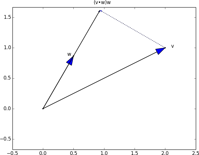
Figure 4-2. The dot product as vector projection
Using this, it’s easy to compute a vector’s sum of squares:
defsum_of_squares(v:Vector)->float:"""Returns v_1 * v_1 + ... + v_n * v_n"""returndot(v,v)assertsum_of_squares([1,2,3])==14# 1 * 1 + 2 * 2 + 3 * 3
which we can use to compute its magnitude (or length):
importmathdefmagnitude(v:Vector)->float:"""Returns the magnitude (or length) of v"""returnmath.sqrt(sum_of_squares(v))# math.sqrt is square root functionassertmagnitude([3,4])==5
We now have all the pieces we need to compute the distance between two vectors, defined as:
In code:
defsquared_distance(v:Vector,w:Vector)->float:"""Computes (v_1 - w_1) ** 2 + ... + (v_n - w_n) ** 2"""returnsum_of_squares(subtract(v,w))defdistance(v:Vector,w:Vector)->float:"""Computes the distance between v and w"""returnmath.sqrt(squared_distance(v,w))
This is possibly clearer if we write it as (the equivalent):
defdistance(v:Vector,w:Vector)->float:returnmagnitude(subtract(v,w))
That should be plenty to get us started. We’ll be using these functions heavily throughout the book.
Matrices
A matrix is a two-dimensional collection of numbers. We will represent matrices as lists of lists, with each inner list having the same size and representing a row of the matrix. If A is a matrix, then A[i][j] is the element in the ith row and the jth column. Per mathematical convention, we will frequently use capital letters to represent matrices. For example:
# Another type aliasMatrix=List[List[float]]A=[[1,2,3],# A has 2 rows and 3 columns[4,5,6]]B=[[1,2],# B has 3 rows and 2 columns[3,4],[5,6]]
Note
In mathematics, you would usually name the first row of the matrix “row 1” and the first column “column 1.” Because we’re representing matrices with Python lists, which are zero-indexed, we’ll call the first row of a matrix “row 0” and the first column “column 0.”
Given this list-of-lists representation, the matrix A has len(A) rows and len(A[0]) columns, which we consider its shape:
fromtypingimportTupledefshape(A:Matrix)->Tuple[int,int]:"""Returns (# of rows of A, # of columns of A)"""num_rows=len(A)num_cols=len(A[0])ifAelse0# number of elements in first rowreturnnum_rows,num_colsassertshape([[1,2,3],[4,5,6]])==(2,3)# 2 rows, 3 columns
If a matrix has n rows and k columns, we will refer to it as an n × k matrix. We can (and sometimes will) think of each row of an n × k matrix as a vector of length k, and each column as a vector of length n:
defget_row(A:Matrix,i:int)->Vector:"""Returns the i-th row of A (as a Vector)"""returnA[i]# A[i] is already the ith rowdefget_column(A:Matrix,j:int)->Vector:"""Returns the j-th column of A (as a Vector)"""return[A_i[j]# jth element of row A_iforA_iinA]# for each row A_i
We’ll also want to be able to create a matrix given its shape and a function for generating its elements. We can do this using a nested list comprehension:
fromtypingimportCallabledefmake_matrix(num_rows:int,num_cols:int,entry_fn:Callable[[int,int],float])->Matrix:"""Returns a num_rows x num_cols matrixwhose (i,j)-th entry is entry_fn(i, j)"""return[[entry_fn(i,j)# given i, create a listforjinrange(num_cols)]# [entry_fn(i, 0), ... ]foriinrange(num_rows)]# create one list for each i
Given this function, you could make a 5 × 5 identity matrix (with 1s on the diagonal and 0s elsewhere) like so:
defidentity_matrix(n:int)->Matrix:"""Returns the n x n identity matrix"""returnmake_matrix(n,n,lambdai,j:1ifi==jelse0)assertidentity_matrix(5)==[[1,0,0,0,0],[0,1,0,0,0],[0,0,1,0,0],[0,0,0,1,0],[0,0,0,0,1]]
Matrices will be important to us for several reasons.
First, we can use a matrix to represent a dataset consisting of multiple vectors, simply by considering each vector as a row of the matrix. For example, if you had the heights, weights, and ages of 1,000 people, you could put them in a 1,000 × 3 matrix:
data=[[70,170,40],[65,120,26],[77,250,19],# ....]
Second, as we’ll see later, we can use an n × k matrix to represent a linear function that maps k-dimensional vectors to n-dimensional vectors. Several of our techniques and concepts will involve such functions.
Third, matrices can be used to represent binary relationships. In Chapter 1, we represented the edges of a network as a collection of pairs (i, j). An alternative representation would be to create a matrix A such that A[i][j] is 1 if nodes i and j are connected and 0 otherwise.
Recall that before we had:
friendships=[(0,1),(0,2),(1,2),(1,3),(2,3),(3,4),(4,5),(5,6),(5,7),(6,8),(7,8),(8,9)]
We could also represent this as:
# user 0 1 2 3 4 5 6 7 8 9#friend_matrix=[[0,1,1,0,0,0,0,0,0,0],# user 0[1,0,1,1,0,0,0,0,0,0],# user 1[1,1,0,1,0,0,0,0,0,0],# user 2[0,1,1,0,1,0,0,0,0,0],# user 3[0,0,0,1,0,1,0,0,0,0],# user 4[0,0,0,0,1,0,1,1,0,0],# user 5[0,0,0,0,0,1,0,0,1,0],# user 6[0,0,0,0,0,1,0,0,1,0],# user 7[0,0,0,0,0,0,1,1,0,1],# user 8[0,0,0,0,0,0,0,0,1,0]]# user 9
If there are very few connections, this is a much more inefficient representation, since you end up having to store a lot of zeros. However, with the matrix representation it is much quicker to check whether two nodes are connected—you just have to do a matrix lookup instead of (potentially) inspecting every edge:
assertfriend_matrix[0][2]==1,"0 and 2 are friends"assertfriend_matrix[0][8]==0,"0 and 8 are not friends"
Similarly, to find a node’s connections, you only need to inspect the column (or the row) corresponding to that node:
# only need to look at one rowfriends_of_five=[ifori,is_friendinenumerate(friend_matrix[5])ifis_friend]
With a small graph you could just add a list of connections to each node object to speed up this process; but for a large, evolving graph that would probably be too expensive and difficult to maintain.
For Further Exploration
-
Linear algebra is widely used by data scientists (frequently implicitly, and not infrequently by people who don’t understand it). It wouldn’t be a bad idea to read a textbook. You can find several freely available online:
-
Linear Algebra, by Jim Hefferon (Saint Michael’s College)
-
Linear Algebra, by David Cherney, Tom Denton, Rohit Thomas, and Andrew Waldron (UC Davis)
-
If you are feeling adventurous, Linear Algebra Done Wrong, by Sergei Treil (Brown University), is a more advanced introduction.
-
-
All of the machinery we built in this chapter you get for free if you use NumPy. (You get a lot more too, including much better performance.)
Get Data Science from Scratch, 2nd Edition now with the O’Reilly learning platform.
O’Reilly members experience books, live events, courses curated by job role, and more from O’Reilly and nearly 200 top publishers.

