Data Science and Engineering at Enterprise Scale

Chapter 4. Introduction to Machine Learning

Machine learning is a vast subject, and can be daunting at first. Many of its core concepts, however, can be understood with simple examples. These ideas form the basis of our thinking for even the most complex models. We will introduce the basic ideas here (see Table 4-1 for a summary), and will build on them in Chapter 5.

Table 4-1. Basic machine learning terms

Term	Description
Model	The functional form of the prediction. In this chapter, we study the linear model only.
Features	Input variables to the model (x).
Label	Output variable (y). In this chapter, labels are floating-point numbers.
Parameters	The set of numbers ($\mathbf{w}$) that relates the features to the label. Parameters must be discovered from many examples of features and their associated labels.
Linear model	A simple but very useful model where each feature is multiplied by a single parameter. The form of the model is $f(\mathbf{x},\mathbf{w})=w_0+{\sum }_{i=1}^N{w}_i{x}_i$, and is used exclusively in this chapter.
Bias	The parameter in a linear model that does not have a feature associated with it (w0).
Training data	A list of features and associated labels. The data is used to determine the parameters of the model.
Loss function	Also referred to as the objective function. The form of the function to be minimized when determining parameters. The loss function used in this chapter is the least squares function.
Normal equation	A direct solution of the linear model with the least squares objective function. Only a linear model can be solved using this equation.
Numerical optimization	A method for solving for parameters for a given loss function and training dataset. The loss function can be for linear or nonlinear models, but only the linear model is studied in this chapter. The only optimization technique used in this chapter is the gradient descent algorithm.
Gradient descent	The most basic numerical optimization technique. It is an iterative process, where the parameters are incrementally updated by evaluating the gradient of the objective at each step.

Linear Regression as a Machine Learning Model

We will start with the most basic machine learning model, which is linear regression:

$$f(x,w_1,w_0)=w_1·x+w_0$$

In mathematical terms, f(x), a function of the independent variable x, and w₁ and w₀ (the slope and intercept) are the parameters of the model. These parameters are not specified here, but must be determined from a set of example data. The process of using example data to determine parameters was historically referred to as a regression. In machine learning parlance, we refer to the determination of parameters as learning. Let’s see how this is accomplished.

In machine learning, a model like this is used as a prediction of a label based on an input feature. The prediction is f(x), and the feature is x. A linear model with N features would have the form:

$$f(x_1,x_2,...,x_N,w_0,...,w_N)=w_0+w_0+\sum _{i=1}^N{w}_i{x}_i$$

where the variable with no feature associated with it is called the bias term. The prediction is a result of applying the model to an incoming feature set, and is based upon a training set of data. The training set contains a list of features and labels. Labels can, in general, take on discrete values (which leads us more naturally to think of them as labels). For the model studied here, labels are simply floating-point numbers.

The previous equation is often written in the more compact linear algebra notation as:

$$f(\mathbf{x},\mathbf{w})=\mathbf{x}\mathbf{w}$$

where:

$$\mathbf{x}=\begin{array}{cccc}\{1& x_1& ...& x_N\}\end{array}$$

is written as a row vector and $𝐰={\left[\begin{array}{cccc}{w}_0& w_1& ...& w_N\end{array}\right]}^T$ is written as a column vector. The value 1 in the first row of the feature vector is there to account for the intercept.

Defining the Loss Function

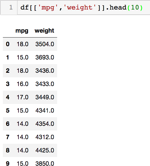
The form of the linear model is defined by the preceding equation, but, as mentioned, the parameters are not specified. We need to determine these parameters by providing example data. We can create a list of M examples as a training set for determining the parameters. The training set will consist of labels, or values $𝐲={\left[\begin{array}{ccc}{y}_1& ...& y_M\end{array}\right]}^T$ and their associated features $𝐗=\left[\begin{array}{ccc}{𝐱}_1& ...& {𝐱}_M\end{array}\right]$. Note that each label entry y_m is a single value, while each row of the matrix X is a row vector x_m, each consisting of N entries. Figure 4-1 shows a training set that we will be using from the notebook.

In the example, the mpg column will be the label column, and the weight column will be the feature. We are using only a single feature for this example (the multivariate case is treated in the notebook).

The loss function, or objective function, is a function that is defined so that the parameters can be determined. In general, the parameters that minimize the loss function will be those that are used. These parameters are completely determined by the data provided and the loss function that is used. The resulting model will have a specific set of parameters $\widehat{\mathbf{w}}$. The loss function that is most commonly used is the mean squared error (MSE), which is defined as:

$$S\left(\mathbf{w}\right)={(\mathbf{y}-\mathbf{X}\mathbf{w})}^T(\mathbf{y}-\mathbf{X}\mathbf{w})$$

and the optimal parameters $\widehat{\mathbf{w}}$ are those that minimize the loss function with respect to $\mathbf{w}$. This idea is expressed mathematically as:

$$\widehat{\mathbf{w}}=\underset{\mathbf{w}}{min}S$$

Figure 4-1. The first few entries of the dataset used for the single feature regression example

The dataset and the objective function provide all of the information needed to define a given model. This basic formulation of the loss function is true for nearly every machine learning model that has labeled data (supervised learning), and this simple linear model provides the conceptual framework that illuminates our understanding of the entire field.

The next step is to solve for the parameters.

Solving for Parameters

A “trick” for linear models: The normal equation

For the simple linear model, a clever solution based on the normal equation can be invoked, which looks as follows (without derivation):

$$\widehat{\mathbf{w}}={\left({\mathbf{X}}^T\mathbf{X}\right)}^{-1}{\mathbf{X}}^T\mathbf{y}$$

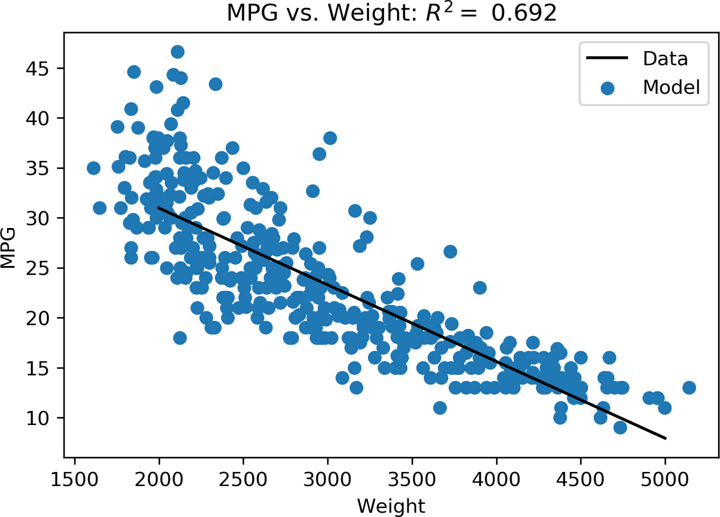
This approach works for any number of features, but is useful only for the linear regression case. Figure 4-2 shows the resulting line generated from this approach, which is described in more depth on GitHub. Any type of model other than a linear regression requires a process called numerical optimization, which is covered in the next section.

Figure 4-2. The best-fitting line through the data as generated with the normal equation

Numerical Optimization, the Workhorse of All Machine Learning

We presented the linear model in some detail because:

• It forms the basis of many other machine learning models.

• The normal equation solution is very convenient and numerically robust.

In fact, the normal equation method provides solutions that are of such high precision that we can use them as “ground truth” solutions. As we explore other methods, it can be very helpful to have a solution with known properties for comparison.

In general, machine learning algorithms result in nonlinear objective functions, which means we need to find another (nonlinear) approach.

The most basic of nonlinear optimization algorithms is the gradient descent algorithm. The idea behind the gradient descent is simple: if the objective function forms a (multidimensional) surface, the gradient of this equation will point in the “downhill” direction. If we follow these downhill steps, we will eventually arrive at a minimum point. There are many caveats to consider here in practice, but the basic concept of an energy landscape can be a very helpful way of thinking about optimization problems. We define the gradient of the objective function as:

$${\left({\nabla }_{\mathbf{w}}S\right)}_i=\frac{\partial S}{\partial w_i}$$

which forms an N-dimensional vector. This vector tells us the slope of the surface. The parameters can be updated to follow the downhill pathway by the following gradient descent step, which takes us from parameter state $\widehat{{\mathbf{w}}_k}$ to ${\widehat{\mathbf{w}}}_{k+1}$:

$${\mathbf{w}}_{k+1}={\mathbf{w}}_k-{\nabla }_{{\mathbf{w}}_k}S·\alpha$$

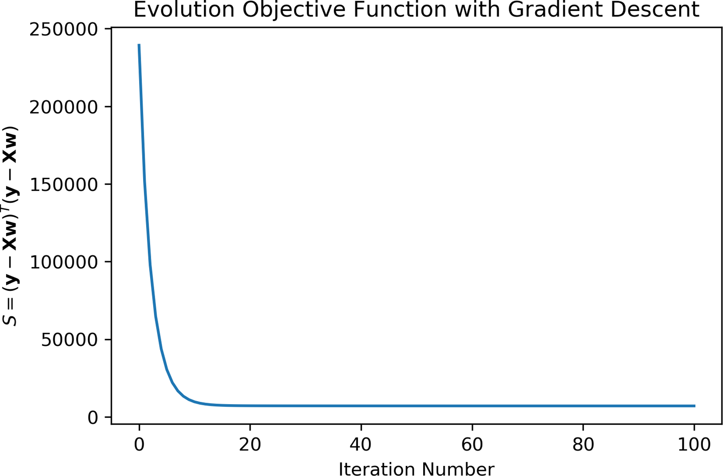
where $\alpha$ is adjusted so that step sizes are optimal. If the steps are too large, we risk leaping across the surface and overstepping the optimal location. If, however, the steps are too small, we may find ourselves taking too many unproductive (and costly) steps. The idea behind each optimization step is that the new parameters ${\widehat{\mathbf{w}}}_{k+1}$ result in a lower loss function. Looking at Figure 4-3, we see that, initially, the objective function is rapidly reduced. Later steps in the process (up to $K=100$) gradually approach a convergent solution. This behavior is typical for a well-behaved optimization process. Had we chosen our $\alpha$ incorrectly, we might not have seen this smooth approach to a stable solution. In fact, you can adjust $\alpha$ yourself in the notebook and see how the behavior changes!

Figure 4-3. Typical convergence behavior of a well-behaved optimization

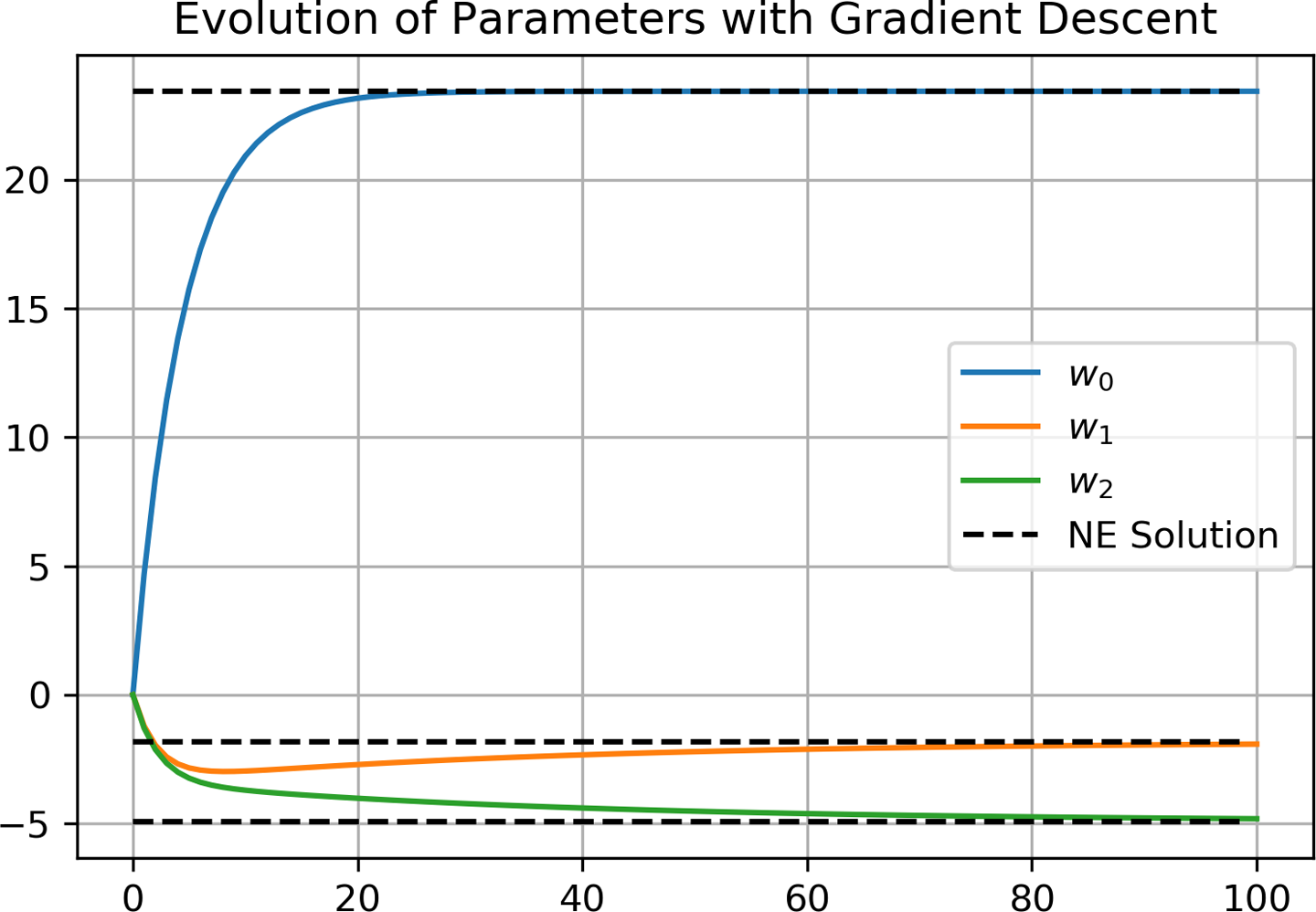
If we look at the evolution of parameters $𝐰={\left[\begin{array}{ccc}{w}_0& w_1& w_2\end{array}\right]}^T$, shown in Figure 4-4, we can see that they gradually approach the ground truth solution from the normal equation. In general, we would not have a solution like this for comparison, and we usually only look at higher-level metrics like the objective function as an indicator of the solution’s fitness. This is one reason why it is so interesting to look at the linear models, because we can make high-resolution comparisons and develop a deeper intuition about how these systems behave.

Note

Don’t forget to watch the evolution of parameters for different values of $\alpha$.

Figure 4-4. Parameters evolve to the ground truth solution as given by the normal equation

Feature Scaling

This well-behaved optimization was not only the result of adjusting the propagation step of gradient descent. It required an additional piece of preprocessing known as feature scaling. Feature scaling is not necessary in the normal equation approach, but is absolutely essential in even the simplest of numerical optimization algorithms. Recall that we like to think of our objective function as a surface. Imagine a surface, like a golf course, where the putting green is an ellipse. Ideally, we would like to have a circular putting green, but an ellipse is okay, right? What about an ellipse that is a foot wide and a mile long? You would want to putt in one direction, but use a driver for the other direction, which would make it hard. Feature scaling has the effect of taking your putting green, no matter how distorted, and making it more symmetric, so that propagation steps are of similar scale no matter what direction you are going.

The most popular way to scale features is standardization scaling, although there are many others. The standardization scaling is given by:

$$x_{j,i}^{\text{'}}=\frac{x_{j,i}-{\mu }_i}{{\sigma }_i}$$

where $x_{j,i}$ is the jth example of ith feature. There are N features and M examples, and the primed notation $x_{j,i}^{\text{'}}$ indicates the scaled feature. The summary variables ${\mu }_i$ and $\sigma$ are the mean and standard deviation of the ith feature across the M examples, respectively.

Without this scaling, you would find yourself adjusting propagation step sizes for each dimension, which would add N more parameters to tune. Also, with this scaling, as well as scaling $\alpha$ by the number of samples, we can obtain more general insights into the range of $\alpha$ that works across many different optimization procedures. The typically recommended range for propagation step size under these conditions is somewhere between 0 and 1 as a result.

Note

Numerical algorithms can be incredibly sensitive to tuning and environments. You can spend an inordinate amount of time tuning the performance of these algorithms by adjusting their parameters or exploring other related gradient descent algorithms.

Letting the Libraries Do Their Job

The optimization, or training, phase of any machine learning or artificial intelligence algorithm is the most time-intensive portion of the entire calculation. This is because it needs to evaluate the objective function as well as the gradient function, and both of these calculations contain M data points of N features. Here, we only needed $K=100$ steps and everything went very quickly, but this can very quickly become a cumbersome problem as $M,N$, and/or $K$ increase.

Furthermore, when the number of data points M becomes very large, the data may need to reside on different machines in your cluster. While this seems like a natural extension, it actually changes the algorithmic approach to favor methods that more efficiently leverage data locality, such as stochastic gradient descent.

While you do want to satisfy yourself that the algorithms are performing as expected, and that you understand the inner workings of the approach, you will increasingly find yourself accessing only the APIs to prewritten algorithms. The frameworks we are discussing in this book are very well validated, highly optimized, and designed with scale in mind.

In general, you can rely on the results of these frameworks, but you may wish to develop ways of comparing results from various approaches to ensure consistency. As these algorithms become more complex, you will want to make higher-level comparisons to ensure that your algorithms are performing as expected. The last section of the notebook contains a simple call to the PySpark linear regresssion algorithm with feature scaling, along with comparisons to the solutions that we studied in detail in earlier sections.

The Data Scientist Has a Job to Do Too

At the end of the notebook, we have looked at the three approaches (normal equation, gradient descent, and MLlib from PySpark). While we may not have all of the details of the results of the PySpark calculation at our immediate disposal, we can generate high-level metrics, such as the R² statistic. This simple comparison can provide enough of a sanity check for both the scientist and engineer to ensure that the calculations are performing as expected.

Recall that you may be comparing results across different frameworks, libraries, and/or languages. Just like a real scientist carrying out a measurement in a laboratory, as a data scientist you must have ways of interpreting the quality of the measurement, even if you may not have a complete understanding of the internals of the calculation. Something as simple as a summary statistic can at least rule out gross errors in inputs and outputs when you are comparing models and methods. If a deeper understanding is required, you can take steps to dive into the finer points of the model being evaluated.

Summary

In this chapter, we have provided the basis for understanding machine learning models. These concepts are surprisingly persistent in even the most complex models, up to and including deep learning models. In Chapter 5, we will build more on these concepts, and see how they are used in classic machine learning examples.