Causal Inference in Python

Chapter 4. The Unreasonable Effectiveness of Linear Regression

In this chapter you’ll add the first major debiasing technique in your causal inference arsenal: linear regression or ordinary least squares (OLS) and orthogonalization. You’ll see how linear regression can adjust for confounders when estimating the relationship between a treatment and an outcome. But, more than that, I hope to equip you with the powerful concept of treatment orthogonalization. This idea, born in linear regression, will come in handy later on when you start to use machine learning models for causal inference.

All You Need Is Linear Regression

Before you skip to the next chapter because “oh, regression is so easy! It’s the first model I learned as a data scientist” and yada yada, let me assure you that no, you actually don’t know linear regression. In fact, regression is one of the most fascinating, powerful, and dangerous models in causal inference. Sure, it’s more than one hundred years old. But, to this day, it frequently catches even the best causal inference researchers off guard.

OLS Research

Don’t believe me? Just take a look at some recently published papers on the topic and you’ll see. A good place to start is the article “Difference-in-Differences with Variation in Treatment Timing,” by Andrew Goodman-Bacon, or the paper “Interpreting OLS Estimands When Treatment Effects Are Heterogeneous” by Tymon Słoczyński, or even the paper “Contamination Bias in Linear Regressions” by Goldsmith-Pinkham et al.

I assure you: not only is regression the workhorse for causal inference, but it will be the one you’ll use the most. Regression is also a major building block for more advanced techniques, like most of the panel data methods (difference-in-differences and two-way fixed effects), machine learning methods (Double/Debiased Machine Learning), and alternative identification techniques (instrumental variables or discontinuity design).

Why We Need Models

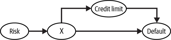
Now that I hopefully convinced you to stay, we can get down to business. To motivate the use of regression, let’s consider a pretty challenging problem in banking and the lending industry in general: understanding the impact of loan amount or credit card limits on default rate. Naturally, increasing someone’s credit card limit will increase (or at least not decrease) the odds of them defaulting on the credit card bill. But, if you look at any banking data, you will see a negative correlation between credit lines and default rate. Obviously, this doesn’t mean that higher lines cause customers to default less. Rather, it simply reflects the treatment assignment mechanism: banks and lending companies offer more credit to customers who have a lower chance of defaulting, as perceived by their underwriting models. The negative correlation you see is the effect of confounding bias:

Of course the bank doesn’t know the inherent risk of default, but it can use proxy variables $X$—like income or credit scores—to estimate it. In the previous chapters, you saw how you could adjust for variables to make the treatment look as good as randomly assigned. Specifically, you saw how the adjustment formula:

$$\begin{array}{c}\hfill ATE=E_x\left\{E\left[Y\right|T=1,X=x]-E[Y|T=0,X=x]\right\},\end{array}$$

which, together with the conditional independence assumption, $(Y_0,Y_1)\perp T|X$, allows you to identify the causal effect.

However, if you were to literally apply the adjustment formula, things can get out of hand pretty quickly. First, you would need to partition your data into segments defined by the feature $X$. This would be fine if you had very few discrete features. But what if there are many of them, with some being continuous? For example, let’s say you know the bank used 10 variables, each with 3 groups, to underwrite customers and assign credit lines. That doesn’t seem a lot, right? Well, it will already amount to 59,049, or $3^{10}$, cells. Estimating the ATE in each of those cells and averaging the result is only possible if you have massive amounts of data. This is the curse of dimensionality, a problem very familiar to most data scientists. In the context of causal inference, one implication of this curse is that a naive application of the adjustment formula will suffer from data sparsity if you have lots of covariates.

Causal Inference Versus Machine Learning Lingo

The literature on machine learning, which is what most data scientists are familiar with, uses different terms from the literature on causal inference, which usually comes from econometrics or epidemiology. So, in the event that you need to translate from one to the other, here are some of the main equivalences you will encounter:

Feature

Covariates or independent variables

Weights

Parameters or coefficients

Target

Outcome or dependent variable

One way out of this dimensionality problem is to assume that the potential outcome can be modeled by something like linear regression, which can interpolate and extrapolate the many individual $X$ defined cells. You can think about linear regression in this context as a dimensionality reduction algorithm. It projects the outcome variable into the $X$ variables and makes the comparison between treatment and control on that projection. It’s quite elegant. But I’m getting ahead of myself. To really (and I mean truly, with every fiber of your heart) understand regression, you have to start small: regression in the context of an A/B test.

Regression in A/B Tests

Pretend you work for an online streaming company, perfecting its recommender system. Your team just finished a new version of this system, with cutting-edge technology and the latest ideas from the machine learning community. While that’s all very impressive, what your manager really cares about is if this new system will increase the watch time of the streaming service. To test that, you decide to do an A/B test. First, you sample a representative but small fraction of your customer base. Then, you deploy the new recommender to a random 1/3 of that sample, while the rest continue to have the old version of the recommender. After a month, you collect the results in terms of average watch time per day:

In [1]: import pandas as pd
        import numpy as np

        data = pd.read_csv("./data/rec_ab_test.csv")
        data.head()
        

	recommender	age	tenure	watch_time
0	challenger	15	1	2.39
1	challenger	27	1	2.32
2	benchmark	17	0	2.74
3	benchmark	34	1	1.92
4	benchmark	14	1	2.47

Since the version of recommender was randomized, a simple comparison of average watch time between versions would already give you the ATE. But then you had to go through all the hassle of computing standard errors to get confidence intervals in order to check for statistical significance. So, what if I told you that you can interpret the results of an A/B test with regression, which will give you, for free, all the inference statistics you need? The idea behind regression is that you’ll estimate the following equation or model:

$$WatchTim{e}_i={\beta }_0+{\beta }_{1}challenge{r}_i+e_i$$

Where $challenger$ is 1 for customers in the group that got the new version of the recommender and zero otherwise. If you estimate this model, the impact of the challenger version will be captured by the estimate of ${\beta }_1$, $\widehat{{\beta }_1}$.

To run that regression model in Python, you can use statsmodels’ formula API. It allows you to express linear models succinctly, using R-style formulas. For example, you can represent the preceding model with the formula 'watch_time ~ C(recommender)'. To estimate the model, just call the method .fit() and to read the results, call .summary() on a previously fitted model:

In [2]: import statsmodels.formula.api as smf

        result = smf.ols('watch_time ~ C(recommender)', data=data).fit()

        result.summary().tables[1]
        

	coef	std err	t	P>|t|	[0.025	0.975]
Intercept	2.0491	0.058	35.367	0.000	1.935	2.163
C(recommender)[T.challenger]	0.1427	0.095	1.501	0.134	–0.044	0.330

In that R-style formula, the outcome variable comes first, followed by a ~. Then, you add the explanatory variables. In this case, you’ll just use the recommender variable, which is categorical with two categories (one for the challenger and one for the old version). You can wrap that variable in C(...) to explicitly state that the column is categorical.

Patsy

The formula syntactic sugar is an incredibly convenient way to do feature engineering. You can learn more about it in the patsy library.

Next, look at the results. First, you have the intercept. This is the estimate for the ${\beta }_0$ parameter in your model. It tells you the expected value of the outcome when the other variables in the model are zero. Since the only other variable here is the challenger indicator, you can interpret the intercept as the expected watch time for those who received the old version of the recommender system. Here, it means that customers spend, on average, 2.04 hours per day watching your streaming content, when with the old version of the recommender system. Finally, looking at the parameter estimate associated with the challenger recommender, $\widehat{{\beta }_1}$, you can see the increase in watch time due to this new version. If $\widehat{{\beta }_0}$ is the estimate for the watch time under the old recommender, $\widehat{{\beta }_0}+\widehat{{\beta }_1}$ tells you the expected watch time for those who got the challenger version. In other words, $\widehat{{\beta }_1}$ is an estimate for the ATE. Due to randomization, you can assign causal meaning to that estimate: you can say that the new recommender system increased watch time by 0.14 hours per day, on average. However, that result is not statistically significant.

Forget the nonsignificant result for a moment, because what you just did was quite amazing. Not only did you estimate the ATE, but also got, for free, confidence intervals and p-values out of it! More than that, you can see for yourself that regression is doing exactly what it supposed to do—estimating $E\left[Y\right|T]$ for each treatment:

In [3]: (data
         .groupby("recommender")
         ["watch_time"]
         .mean())
        

Out[3]: recommender
        benchmark     2.049064
        challenger    2.191750
        Name: watch_time, dtype: float64
        

Just like I’ve said, the intercept is mathematically equivalent to the average watch time for those in the control—the old version of the recommender.

These numbers are identical because, in this case, regression is mathematically equivalent to simply doing a comparison between averages. This also means that $\widehat{{\beta }_1}$ is the average difference between the two groups: $2.191-2.049=0.1427$. OK, so you managed to, quite literally, reproduce group averages with regressions. But so what? It’s not like you couldn’t do this earlier, so what is the real gain here?

Adjusting with Regression

To appreciate the power of regression, let me take you back to the initial example: estimating the effect of credit lines on default. Bank data usually looks something like this, with a bunch of columns of customer features that might indicate credit worthiness, like monthly wage, lots of credit scores provided by credit bureaus, tenure at current company and so on. Then, there is the credit line given to that customer (the treatment in this case) and the column that tells you if a customer defaulted or not—the outcome variable:

In [4]: risk_data = pd.read_csv("./data/risk_data.csv")

        risk_data.head()
        

	wage	educ	exper	married	credit_score1	credit_score2	credit_limit	default
0	950.0	11	16	1	500.0	518.0	3200.0	0
1	780.0	11	7	1	414.0	429.0	1700.0	0
2	1230.0	14	9	1	586.0	571.0	4200.0	0
3	1040.0	15	8	1	379.0	411.0	1500.0	0
4	1000.0	16	1	1	379.0	518.0	1800.0	0

Simulated Data

Once again, I’m building from real-world data and changing it to fit the needs of this chapter. This time, I’m using the wage1 data, curated by professor Jeffrey M. Wooldridge and available in the “wooldridge” R package.

Here, the treatment, credit_limit, has way too many categories. In this situation, it is better to treat it as a continuous variable, rather than a categorical one. Instead of representing the ATE as the difference between multiple levels of the treatment, you can represent it as the derivative of the expected outcome with respect to the treatment:

$$ATE=\frac{\partial }{\partial t}E\left[y\right|t]$$

Don’t worry if this sounds fancy. It simply means the amount you expect the outcome to change given a unit increase in the treatment. In this example, it represents how much you expect the default rate to change given a 1 USD increase in credit lines.

One way to estimate such a quantity is to run a regression. Specifically, you can estimate the model:

$${\mathit{Default}}_i={\beta }_0+{\beta }_1{\mathrm{limit}}_i+e_i,$$

and the estimate ${\widehat{\beta }}_1$ can be interpreted as the amount you expect risk to change given a 1 USD increase in limit. This parameter has a causal interpretation if the limit was randomized. But as you know very well that is not the case, as banks tend to give higher lines to customers who are less risky. In fact, if you run the preceding model, you’ll get a negative estimate for ${\beta }_1$:

In [5]: model = smf.ols('default ~ credit_limit', data=risk_data).fit()
        model.summary().tables[1]
        

	coef	std err	t	P>|t|	[0.025	0.975]
Intercept	0.2192	0.004	59.715	0.000	0.212	0.226
credit_limit	–2.402e–05	1.16e–06	–20.689	0.000	–2.63e–05	–2.17e–05

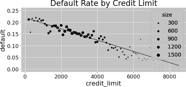
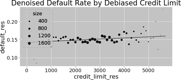
That is not at all surprising, given the fact that the relationship between risk and credit limit is negative, due to confounding. If you plot the fitted regression line alongside the average default by credit limit, you can clearly see the negative trend:

To adjust for this bias, you could, in theory, segment your data by all the confounders, run a regression of default on credit lines inside each segment, extract the slope parameter, and average the results. However, due to the curse of dimensionality, even if you try to do that for a moderate number of confounders—both credit scores—you will see that there are cells with only one sample, making it impossible for you to run your regression. Not to mention the many cells that are simply empty:

In [6]: risk_data.groupby(["credit_score1", "credit_score2"]).size().head()
        

Out[6]: credit_score1  credit_score2
        34.0           339.0            1
                       500.0            1
        52.0           518.0            1
        69.0           214.0            1
                       357.0            1
        dtype: int64
        

Thankfully, once more, regression comes to your aid here. Instead of manually adjusting for the confounders, you can simply add them to the model you’ll estimate with OLS:

$${\mathit{Default}}_i={\beta }_0+{\beta }_1{\mathrm{limit}}_i+{\theta \mathbf{X}}_i+e_i,$$

Here, $𝐗$ is a vector of confounder variables and $\theta$ is the vector of parameters associated with those confounders. There is nothing special about $\theta$ parameters. They behave exactly like ${\beta }_1$. I’m representing them differently because they are just there to help you get an unbiased estimate for ${\beta }_1$. That is, you don’t really care about their causal interpretation (they are technically called nuisance parameters).

In the credit example, you could add the credit scores and wage confounders to the model. It would look like this:

$${\mathit{Default}}_i={\beta }_0+{\beta }_1{\mathrm{limit}}_i+{\theta }_1{\mathrm{wage}}_i+{\theta }_2\mathrm{creditScore}{1}_i+{\theta }_3\mathrm{creditScore}{2}_i+e_i,$$

I’ll get into more details about how including variables in the model will adjust for confounders, but there is a very easy way to see it right now. The preceding model is a model for $E\left[y\right|t,X]$. Recall that you want $\frac{\partial }{\partial t}E\left[y\right|t,X]$. So what happens if you differentiate the model with respect to the treatment—credit limit? Well, you simply get ${\beta }_1$! In a sense, ${\beta }_1$ can be seen as the partial derivative of the expected value of default with respect to credit limit. Or, more intuitively, it can be viewed as how much you should expect default to change, given a small increase in credit limit, while holding fixed all other variables in the model. This interpretation already tells you a bit of how regression adjusts for confounders: it holds them fixed while estimating the relationship between the treatment and the outcome.

To see this in action, you can estimate the preceding model. Just add some confounders and, like some kind of magic, the relationship between credit lines and default becomes positive!

In [7]: formula = 'default ~ credit_limit + wage+credit_score1+credit_score2'
        model = smf.ols(formula, data=risk_data).fit()
        model.summary().tables[1]
        

	coef	std err	t	P>|t|	[0.025	0.975]
Intercept	0.4037	0.009	46.939	0.000	0.387	0.421
credit_limit	3.063e–06	1.54e–06	1.987	0.047	4.16e–08	6.08e–06
wage	–8.822e-05	6.07e–06	–14.541	0.000	–0.000	–7.63e–05
credit_score1	–4.175e–05	1.83e–05	–2.278	0.023	–7.77e–05	–5.82e–06
credit_score2	–0.0003	1.52e–05	–20.055	0.000	–0.000	–0.000

Don’t let the small estimate of ${\beta }_1$ fool you. Recall that limit is in the scales of 1,000s while default is either 0 or 1. So it is no surprise that increasing lines by 1 USD will increase expected default by a very small number. Still, that number is statistically significant and tells you that risk increases as you increase credit limit, which is much more in line with your intuition on how the world works.

Hold that thought because you are about to explore it more formally. It’s finally time to learn one of the greatest causal inference tools of all: the Frisch-Waugh-Lovell (FWL) theorem. It’s an incredible way to get rid of bias, which is unfortunately seldom known by data scientists. FWL is a prerequisite to understand more advanced debiasing methods, but the reason I find it most useful is that it can be used as a debiasing pre-processing step. To stick to the same banking example, imagine that many data scientists and analysts in this bank are trying to understand how credit limit impacts (causes) lots of different business metrics, not just risk. However, only you have the context about how the credit limit was assigned, which means you are the only expert who knows what sort of biases plague the credit limit treatment. With FWL, you can use that knowledge to debias the credit limit data in a way that it can be used by everyone else, regardless of what outcome variable they are interested in. The Frisch-Waugh-Lovell theorem allows you to separate the debiasing step from the impact estimation step. But in order to learn it, you must first quickly review a bit of regression theory.

Regression Theory

I don’t intend to dive too deep into how linear regression is constructed and estimated. However, a little bit of theory will go a long way in explaining its power in causal inference. First of all, regression solves the best linear prediction problem. Let ${\beta }^{*}$ be a vector of parameters:

${\beta }^{*}=\underset{\beta }{argmin}E\left[{(Y_i-X_i^{\text{'}}\beta )}^2\right]$

Linear regression finds the parameters that minimize the mean squared error (MSE). If you differentiate it and set it to zero, you will find that the linear solution to this problem is given by:

${\beta }^{*}=E{\left[X^{\text{'}}X\right]}^{-1}E\left[X^{\text{'}}Y\right]$

You can estimate this beta using the sample equivalent:

$\widehat{\beta }={\left(X^{\text{'}}X\right)}^{-1}{X}^{\text{'}}Y$

But don’t take my word for it. If you are one of those who understand code better than formulas, try for yourself. In the following code, I’m using the algebraic solution to OLS to estimate the parameters of the model you just saw (I’m adding the intercept as the final variables, so the first parameter estimate will be $\widehat{{\beta }_1}$):

In [8]: X_cols = ["credit_limit", "wage", "credit_score1", "credit_score2"]
        X = risk_data[X_cols].assign(intercep=1)
        y = risk_data["default"]

        def regress(y, X): 
            return np.linalg.inv(X.T.dot(X)).dot(X.T.dot(y))

        beta = regress(y, X)
        beta
        

Out[8]: array([ 3.062e-06, -8.821e-05, -4.174e-05, -3.039e-04, 4.0364-01])
        

If you look back a bit, you will see that these are the exact same numbers you got earlier, when estimating the model with the ols function from statsmodels.

Assign

I tend to use the method .assign() from pandas quite a lot. If you are not familiar with it, it just returns a new data frame with the newly created columns passed to the method:

new_df = df.assign(new_col_1 = 1,
                   new_col_2 = df["old_col"] + 1)

new_df[["old_col", "new_col_1", "new_col_2"]].head()

   old_col  new_col_1  new_col_2
0        4          1          5
1        9          1         10
2        8          1          9
3        0          1          1
4        6          1          7

Single Variable Linear Regression

The $\widehat{\beta }$ formula from the previous section is pretty general. However, it pays off to study the case where you only have one regressor. In causal inference, you often want to estimate the causal impact of a variable $T$ on an outcome $Y$. So, you use regression with this single variable to estimate this effect.

With a single regressor variable $T$, the parameter associated to it will be given by:

$\widehat{\tau }={\displaystyle \frac{Cov(Y_i,T_i)}{Var\left(T_i\right)}}={\displaystyle \frac{E\left[(T_i-\overline{T})(Y_i-\overline{Y})\right]}{E\left[{(T_i-\overline{T})}^2\right]}}$

If $T$ is randomly assigned, ${\beta }_1$ is the ATE. Importantly, with this simple formula, you can see what regression is doing. It’s finding out how the treatment and outcome move together (as expressed by the covariance in the numerator) and scaling this by units of the treatment, which is achieved by dividing by the variance of the treatment.

Note

You can also tie this to the general formula. Covariance is intimately related to dot products, so you can pretty much say that $X^{\text{'}}X$ takes the role of the denominator in the covariance/variance formula, while $X^{\text{'}}y$ takes the role of the numerator.

Multivariate Linear Regression

Turns out there is another way to see multivariate linear regression, beyond the general formula you saw earlier. This other way sheds some light into what regression is doing.

If you have more than one regressor, you can extend the one variable regression formula to accommodate that. Let’s say those other variables are just auxiliary and that you are truly interested in estimating the parameter $\tau$ associated to $T$:

$y_i={\beta }_0+\tau T_i+{\beta }_1{X}_{1i}+...+{\beta }_k{X}_{ki}+u_i$

$\tau$ can be estimated with the following formula:

$\widehat{\tau }={\displaystyle \frac{Cov(Y_i,\widetilde{T_i})}{Var\left(\widetilde{T_i}\right)}}$

where $\widetilde{T_i}$ is the residual from a regression of $T_i$ on all of the other covariates $X_{1i}+...+X_{ki}$.

Now, let’s appreciate how cool this is. It means that the coefficient of a multivariate regression is the bivariate coefficient of the same regressor after accounting for the effect of other variables in the model. In causal inference terms, $\tau$ is the bivariate coefficient of $T$ after having used all other variables to predict it.

This has a nice intuition behind it. If you can predict $T$ using other variables, it means it’s not random. However, you can make $T$ look as good as random once you control for the all the confounder variables $X$. To do so, you can use linear regression to predict it from the confounder and then take the residuals of that regression $\tilde{T}$. By definition, $\tilde{T}$ cannot be predicted by the other variables $X$ that you’ve already used to predict $T$. Quite elegantly, $\tilde{T}$ is a version of the treatment that is not associated (uncorrelated) with any other variable in $X$.

I know this is a mouthful, but it is just amazing. In fact, it is already the work of the FWL theorem that I promised to teach you. So don’t worry if you didn’t quite get this multivariate regression part, as you are about to review it in a much more intuitive and visual way.

Frisch-Waugh-Lovell Theorem and Orthogonalization

FWL-style orthogonalization is the first major debiasing technique you have at your disposal. It’s a simple yet powerful way to make nonexperimental data look as if the treatment has been randomized. FWL is mostly about linear regression; FWL-style orthogonalization has been expanded to work in more general contexts, as you’ll see in Part III. The Frisch-Waugh-Lovell theorem states that a multivariate linear regression model can be estimated all at once or in three separate steps. For example, you can regress default on credit_limit, wage, credit_score1, credit_score2, just like you already did:

In [9]: formula = 'default ~ credit_limit + wage+credit_score1+credit_score2'
        model = smf.ols(formula, data=risk_data).fit()
        model.summary().tables[1]
        

	coef	std err	t	P>|t|	[0.025	0.975]
Intercept	0.4037	0.009	46.939	0.000	0.387	0.421
credit_limit	3.063e–06	1.54e–06	1.987	0.047	4.16e–08	6.08e–06
wage	–8.822e–05	6.07e–06	–14.541	0.000	–0.000	–7.63e–05
credit_score1	–4.175e–05	1.83e–05	–2.278	0.023	-–7.77e–05	-5.82e–06
credit_score2	–0.0003	1.52e–05	–20.055	0.000	–0.000	–0.000

But, according to FWL, you can also break down this estimation into:

1. A debiasing step, where you regress the treatment $T$ on confounders $X$ and obtain the treatment residuals $\tilde{T}=T-\widehat{T}$

2. A denoising step, where you regress the outcome $Y$ on the confounder variables $X$ and obtain the outcome residuals $\tilde{Y}=Y-\widehat{Y}$

3. An outcome model where you regress the outcome residual $\tilde{Y}$ on the treatment residual $\tilde{T}$ to obtain an estimate for the causal effect of $T$ on $Y$

Not surprisingly, this is just a restatement of the formula you just saw in “Multivariate Linear Regression”. The FWL theorem states an equivalence in estimation procedures with regression models. It also says that you can isolate the debiasing component of linear regression, which is the first step outlined in the preceding list.

To get a better intuition on what is going on, let’s break it down step by step.

Debiasing Step

Recall that, initially, due to confounding bias, your data looked something like this, with default trending downward with credit line:

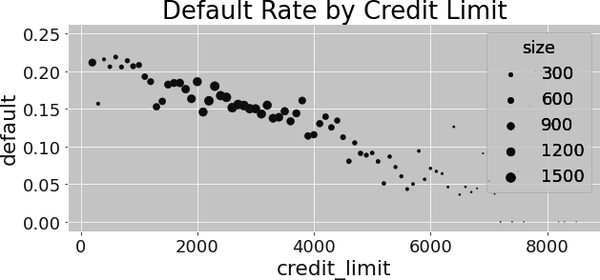
According to the FWL theorem, you can debias this data by fitting a regression model to predict the treatment—the credit limit—from the confounders. Then, you can take the residual from this model: ${\widetilde{line}}_i=lin{e}_i-{\widehat{line}}_i$. This residual can be viewed as a version of the treatment that is uncorrelated with the variables used in the debiasing model. That’s because, by definition, the residual is orthogonal to the variables that generated the predictions.

This process will make $\widetilde{line}$ centered around zero. Optionally, you can add back the average treatment, $\overline{line}$:

$${\widetilde{line}}_i=lin{e}_i-{\widehat{line}}_i+\overline{line}$$

This is not necessary for debiasing, but it puts $\widetilde{line}$ in the same range as the original $line$, which is better for visualization purposes:

In [10]: debiasing_model = smf.ols(
             'credit_limit ~ wage + credit_score1  + credit_score2',
             data=risk_data
         ).fit()

         risk_data_deb = risk_data.assign(
             # for visualization, avg(T) is added to the residuals
             credit_limit_res=(debiasing_model.resid 
                               + risk_data["credit_limit"].mean())
         )
         

If you now run a simple linear regression, where you regress the outcome, $risk$, on the debiased or residualized version of the treatment, $\widetilde{line}$, you’ll already get the effect of credit limit on risk while controlling for the confounders used in the debiasing model. The parameter estimate you get for ${\beta }_1$ here is exactly the same as the one you got earlier by running the complete model, where you’ve included both treatment and confounders:

In [11]: model_w_deb_data = smf.ols('default ~ credit_limit_res',
                                    data=risk_data_deb).fit()

         model_w_deb_data.summary().tables[1]
         

	coef	std err	t	P>|t|	[0.025	0.975]
Intercept	0.1421	0.005	30.001	0.000	0.133	0.151
credit_limit_res	3.063e-06	1.56e–06	1.957	0.050	–4.29e–09	6.13e–06

Alternative Coefficient Formula

The fact that you only need to residualize the treatment suggests a simpler way of rewriting the regression coefficient formula. In the single variable case, instead of using the covariance of $Y$ and $T$ over the variance of $T$, you can use

$${\beta }_1={\displaystyle \frac{E\left[(T_i-\overline{T})y_i\right]}{E\left[{(T_i-\overline{T})}^2\right]}}.$$

In the multivariate case, this would be

$${\beta }_1={\displaystyle \frac{E\left[(T_i-E\left[T\right|X])y_i\right]}{E\left[Var\left(T\right|X)\right]}}.$$

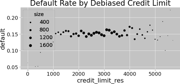
There is a difference, though. Look at the p-value. It is a bit higher than what you got earlier. That’s because you are not applying the denoising step, which is responsible for reducing variance. Still, with only the debiasing step, you can already get the unbiased estimate of the causal impact of credit limit on risk, given that all the confounders were included in the debiasing model.

You can also visualize what is going on by plotting the debiased version of credit limit against default rate. You’ll see that the relationship is no longer downward sloping, as when the data was biased:

Denoising Step

While the debiasing step is crucial to estimate the correct causal effect, the denoising step is also nice to have, although not as important. It won’t change the value of your treatment effect estimate, but it will reduce its variance. In this step, you’ll regress the outcome on the covariates that are not the treatment. Then, you’ll get the residual for the outcome ${\widetilde{\mathit{default}}}_i={\mathit{default}}_i-{\widehat{\mathit{default}}}_i$.

Once again, for better visualization, you can add the average default rate to the denoised default variable for better visualization purposes:

$${\widetilde{\mathit{default}}}_i={\mathit{default}}_i-{\widehat{\mathit{default}}}_i+\overline{\mathit{default}}$$

In [12]: denoising_model = smf.ols(
             'default ~ wage + credit_score1  + credit_score2',
             data=risk_data_deb
         ).fit()

         risk_data_denoise = risk_data_deb.assign(
             default_res=denoising_model.resid + risk_data_deb["default"].mean()
         )
         

Standard Error of the Regression Estimator

Since we are talking about noise, I think it is a good time to see how to compute the regression standard error. The SE of the regression parameter estimate is given by the following formula:

$$SE\left(\widehat{\beta }\right)={\displaystyle \frac{\sigma \left(\widehat{ϵ}\right)}{\sigma \left(\tilde{T}\right)\sqrt{n-DF}}},$$

where $\widehat{ϵ}$ is the residual from the regression model and $DF$ is the model’s degree of freedom (number of parameters estimated by the model). If you prefer to see this in code, here it is:

In [13]: model_se = smf.ols(
        'default ~ wage + credit_score1  + credit_score2',
        data=risk_data
    ).fit()

    print("SE regression:", model_se.bse["wage"])

    
    model_wage_aux = smf.ols(
        'wage ~ credit_score1 + credit_score2',
        data=risk_data
    ).fit()

    # subtract the degrees of freedom - 4 model parameters - from N.
    se_formula = (np.std(model_se.resid)
               /(np.std(model_wage_aux.resid)*np.sqrt(len(risk_data)-4)))

    print("SE formula:   ", se_formula)
    

Out[13]: SE regression: 5.364242347548197e-06
         SE formula:    5.364242347548201e-06
         

This formula is nice because it gives you further intuition about regression in general and the denoising step in particular. First, the numerator tells you that the better you can predict the outcome, the smaller the residuals will be and, hence, the lower the variance of the estimate. This is very much what the denoising step is all about. It also tells you that if the treatment explains the outcome a lot, its parameter estimate will also have a smaller standard error.

Interestingly, the error is also inversely proportional to the variance of the (residualized) treatment. This is also intuitive. If the treatment varies a lot, it will be easier to measure its impact. You’ll learn more about this in “Noise Inducing Control”.

Experiments with Continuous Treatments

The standard error formula can also be useful if you plan to design an experiment where you care to measure the effect as the parameter estimate from a regression. This is a good idea if the treatment you want to randomize is continuous. In this case, the standard error formula can be approximated by:

$$SE\approx \frac{\sigma \left(y\right)}{\sigma \left(T\right)\sqrt{n-2}}$$

This approximation is conservative in the case of a single variable regression model, since $\sigma \left(y\right)\ge \sigma \left(\widehat{e}\right)$, because the treatment might explain a bit of the outcome. Then, you can take this standard error and plug in the sample size calculation formula from Chapter 2. Importantly, designing this test has the additional complexity of choosing a sampling distribution from $T$, which can also affect the standard error via $\sigma \left(T\right)$.

Final Outcome Model

With both residuals, $\tilde{Y}$ and $\tilde{T}$, you can run the final step outlined by the FWL theorem—just regress $\tilde{Y}$ on $\tilde{T}$:

In [14]: model_w_orthogonal = smf.ols('default_res ~ credit_limit_res',
                                      data=risk_data_denoise).fit()

         model_w_orthogonal.summary().tables[1]
         

	coef	std err	t	P>|t|	[0.025	0.975]
Intercept	0.1421	0.005	30.458	0.000	0.133	0.151
credit_limit_res	3.063e–06	1.54e–06	1.987	0.047	4.17e–08	6.08e–06

The parameter estimate for the treatment is exactly the same as the one you got in both the debiasing step and when running the regression model with credit limit plus all the other covariates. Additionally, the standard error and p-value are now also just like when you first ran the model, with all the variables included. This is the effect of the denoising step.

Of course, you can also plot the relationship between the debiased treatment with the denoised outcome, alongside the predictions from the final model to see what is going on:

FWL Summary

I don’t know if you can already tell, but I really like illustrative figures. Even if they don’t reflect any real data, they can be quite useful to visualize what is going on behind some fairly technical concept. It wouldn’t be different with FWL. So to summarize, consider that you want to estimate the relationship between a treatment $T$ and an outcome $Y$ but you have some confounder $X$. You plot the treatment on the x-axis, the outcome on the y-axis, and the confounder as the color dimension. You initially see a negative slope between treatment and outcome, but you have strong reasons (some domain knowledge) to believe that the relationship should be positive, so you decide to debias the data.

To do that, you first estimate $E\left[T\right|X]$ using linear regression. Then, you construct a debiased version of the treatment: $T-E\left[T\right|X]$ (see Figure 4-1). With this debiased treatment, you can already see the positive relationship you were hoping to find. But you still have a lot of noise.

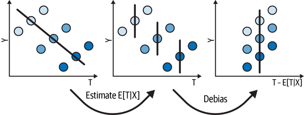
Figure 4-1. How orthogonalization removes bias

To deal with the noise, you estimate $E\left[Y\right|X]$, also using a regression model. Then, you construct a denoised version of the outcome: $Y-E\left[Y\right|X]$ (see Figure 4-2). You can view this denoised outcome as the outcome after you’ve accounted for all the variance in it that was explained by $X$. If $X$ explains a lot of the variance in $Y$, the denoised outcome will be less noisy, making it easier to see the relationship you really care about: that between $T$ and $Y$.

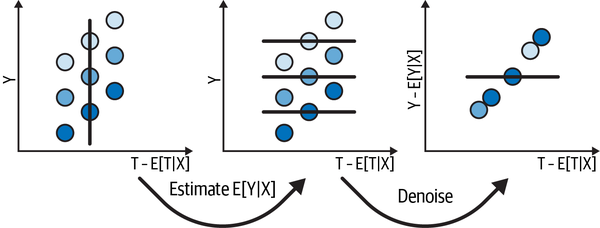
Figure 4-2. How orthogonalization removes noise

Finally, after both debiasing and denoising, you can clearly see a positive relationship between $T$ and $Y$. All there is left to do is fit a final model to this data:

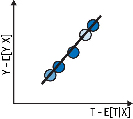
This final regression will have the exact same slope as the one where you regress $Y$ on $T$ and $X$ at the same time.

Debiasing and the Intercept

One word of caution, though. In causal inference, you are mostly concerned with the slope of this regression line, since the slope is a linear approximation to the effect of the continuous treatment, $\frac{\partial }{\partial t}E\left[y\right|t]$. But, if you also care about the intercept—for instance, if you are trying to do counterfactual predictions—you should know that debiasing and denoising makes the intercept equal to zero.

Regression as an Outcome Model

Throughout this section I emphasized how regression works mostly by orthogonalizing the treatment. However, you can also see regression as a potential outcome imputation technique. Suppose that the treatment is binary. If regression of $Y$ on $X$ in the control population ($T=0$) yields good approximation to $E\left[Y_0\right|X]$, then you can use that model to impute $Y_0$ and estimate the ATT:

$$ATT=\frac{1}{N_1}\sum \mathbb{1}(T_i=1)\left(Y_i-{\widehat{\mu }}_0\left(X_i\right)\right),$$

where $N_1$ is the number of treated units.

Indicator Function

Throughout this book, I’ll use $\mathbb{1}(.)$ to represent the indicator function. This function returns 1 when the argument inside it evaluates to true and zero otherwise.

A similar argument can be made to show that if regression on the treated units can model $E\left[Y_1\right|X]$, you can use it to estimate the average effect on the untreated. If you put these two arguments side by side, you can estimate the ATE as follows:

$$ATE=\frac{1}{N}\sum \left({\widehat{\mu }}_1\left(X_i\right)-{\widehat{\mu }}_0\left(X_i\right)\right)$$

This estimator will impute both potential outcomes for all units. It is equivalent to regressing $Y$ on both $X$ and $T$ and reading the parameter estimate on $T$.

Alternatively, you can impute just the potential outcomes that are missing:

$$ATE=\frac{1}{N}\sum \left(\mathbb{1}(T_i=1)\left[Y_i-{\widehat{\mu }}_0\left(X_i\right)\right]+\mathbb{1}(T_i=0)\left[{\widehat{\mu }}_1\left(X_i\right)-Y_i\right]\right)$$

When $T$ is continuous, this is a bit harder to conceptualize, but you can understand regression as imputing the whole treatment response function, which involves imputing the potential outcomes $Y\left(t\right)$ as if it was a line.

The fact that regression works if it can either correctly estimate $E\left[T\right|X]$ for orthogonalization or correctly estimate the potential outcomes $E\left[Y_t\right|X]$ grants it doubly robust properties, something you’ll explore further in Chapter 5. Seeing regression through this lens will also be important when you learn about difference-in-differences in Part IV.

Public or Private Schools?

In the book Mastering Metrics (Princeton University Press), Angrist and Pischke show how regression can be used to adjust for the bias when estimating the impact of going to private schools on one’s income. Graduates of private school often make more money than those of public school, but it’s hard to say how much of this relationship is causal. For instance, your parents’ income might confound the relationship, as kids of richer families are both more likely to go to private schools and to earn more. Similarly, since private schools are very selective, it could be that they take in only the students who would already be better off anyway.

So much so that a naive regression of income on a private school dummy is almost sure to return a positive effect. In other words, estimating the following model would give you a positive and significant $\widehat{{\beta }_1}$:

$$incom{e}_i={\delta }_0+{\beta }_{1}private+e_i$$

What Angrist and Pischke show, however, is that if you adjust for SAT score and parents’ income, the measured impact decreases. That is, if you augment the model with these two variables, your $\widehat{{\beta }_1}$ will be smaller, compared to the one you would get with the short model:

$$incom{e}_i={\delta }_0+{\beta }_{1}private+{\delta }_{1}SA{T}_i+{\delta }_{2}ParentIn{c}_i+e_i$$

Still, after running a regression with parent income, the effect of private schools remained positive and significant, at least in the dataset used by the authors. However, one final set of controls managed to make the relationship insignificant. The authors included the average SAT of the school the students applied to (regardless of them being accepted). This can be interpreted as a proxy for ambition:

$$\begin{array}{c}\hfill \begin{array}{cc}\hfill incom{e}_i& ={\delta }_0+{\beta }_{1}private+{\delta }_{1}SA{T}_i+{\delta }_{2}ParentIn{c}_i\hfill \\ & +{\delta }_{3}AvgSATSchoo{l}_i+e_i\hfill \end{array}\end{array}$$

Once they added the ambition proxy controls, the estimated $\widehat{{\beta }_1}$ became insignificant. Interestingly, keeping only those controls and dropping the SAT and parents’ income controls still resulted in a nonsignificant estimate. This indicates that, given your ambition level, it doesn’t matter if you go to a public or private school, at least in terms of your earnings:

Positivity and Extrapolation

Since regression models the potential outcome as a parametric function, it allows for extrapolation outside the region where you have data on all treatment levels. This can be a blessing or a curse. It all depends on whether the extrapolation is reasonable. For example, consider that you have to estimate a treatment effect in a dataset with low overlap. Call it Dataset 1. Dataset 1 has no control units for high values of a covariate $x$ and no treated units for low values of that same covariate. If you use regression to estimate the treatment effect on this data, it will impute $Y_0$ and $Y_1$ as shown by the lines in the first plot:

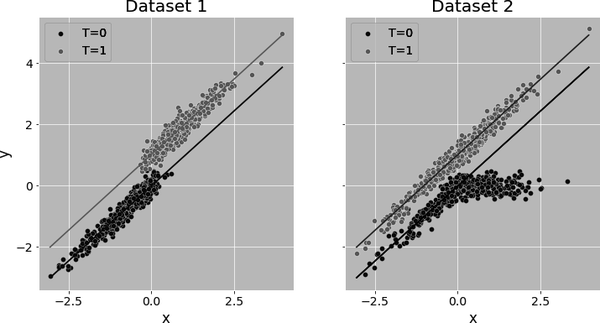
This is fine, so long as the same relationship between $Y_0$ and $x$ you’ve fitted in the control for low levels of $x$ is also valid for high values of $x$ and that the $Y_1$ you’ve fitted on the treated also extrapolates well to low levels of $x$. Generally, if the trends in the outcome where you do have overlap look similar across the covariate space, a small level of extrapolation becomes less of an issue.

However, too much extrapolation is always dangerous. Let’s suppose you’ve estimated the effect on Dataset 1, but then you collect more data, now randomizing the treatment. On this new data, call it Dataset 2, you see that the effect gets larger and larger for positive values of $x$. Consequently, if you evaluate your previous fit on this new data, you’ll realize that you grossly underestimated the true effect of the treatment. This goes to show that you can never really know what will happen to the treatment effect in a region where you don’t have positivity. You might choose to trust your extrapolations for those regions, but that is not without risk.

Nonlinearities in Linear Regression

Up until this point, the treatment response curve seemed pretty linear. It looked like an increase in credit line caused a constant increase in risk, regardless of the credit line level. Going from a line of 1,000 to 2,000 seemed to increase risk about the same as going from a line of 2,000 to 3,000. However, you are likely to encounter situations where this won’t be the case.

As an example, consider the same data as before, but now your task is to estimate the causal effect of credit limit on credit card spend:

In [15]: spend_data = pd.read_csv("./data/spend_data.csv")

         spend_data.head()
         

	wage	educ	exper	married	credit_score1	credit_score2	credit_limit	spend
0	950.0	11	16	1	500.0	518.0	3200.0	3848
1	780.0	11	7	1	414.0	429.0	1700.0	3144
2	1230.0	14	9	1	586.0	571.0	4200.0	4486
3	1040.0	15	8	1	379.0	411.0	1500.0	3327
4	1000.0	16	1	1	379.0	518.0	1800.0	3508

And for the sake of simplicity, let’s consider that the only confounder you have here is wage (assume that is the only information the bank uses when deciding the credit limit). The causal graph of this process looks something like this:

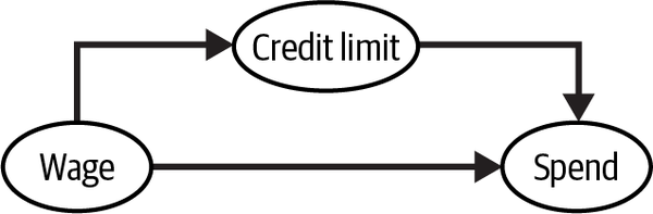
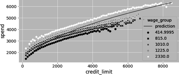
As a result, you have to condition on wage to identify the effect of credit lines on spending. If you want to use orthogonalization to estimate this effect, you can say that you need to debias credit lines by regressing it on wage and getting the residuals. Nothing new so far. But there is a catch. If you plot spend by credit lines for multiple wage levels, you can clearly see that the relationship is not linear:

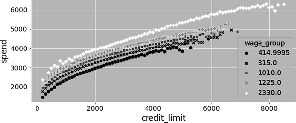
Rather, the treatment response curve seems to have some sort of concavity to it: the higher the credit limit, the lower the slope of this curve. Or, in causal inference language, since slopes and causal effects are intimately related, you can also say that the effect of lines on spend diminishes as you increase lines: going from a line of 1,000 to 2,000 increases spend more than going from 2,000 to 3,000.

Linearizing the Treatment

To deal with that, you first need to transform the treatment into something that does have a linear relationship with the outcome. For instance, you know that the relationship seems concave, so you can try to apply some concave function to lines. Some good candidates to try out are the log function, the square root function, or any function that takes credit lines to the power of a fraction.

In this case, let’s try the square root:

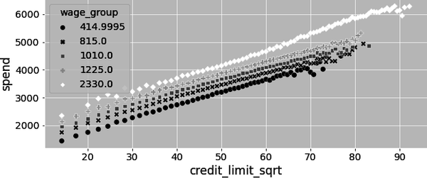
Now we are getting somewhere! The square root of the credit line seems to have a linear relationship with spend. It’s definitely not perfect. If you look very closely, you can still see some curvature. But it might just do for now.

I’m sad to say that this process is fairly manual. You have to try a bunch of stuff and see what linearizes the treatment better. Once you find something that you are happy with, you can apply it when running a linear regression model. In this example, it means that you will be estimating the model:

$$spen{d}_i={\beta }_0+{\beta }_1{\sqrt{line}}_i+e_i$$

and your causal parameter is ${\beta }_1$.

This model can be estimated with statsmodels, by using the NumPy square root function directly in the formula:

In [16]: model_spend = smf.ols(
             'spend ~ np.sqrt(credit_limit)',data=spend_data
         ).fit()

         model_spend.summary().tables[1]
         

	coef	std err	t	P>|t|	[0.025	0.975]
Intercept	493.0044	6.501	75.832	0.000	480.262	505.747
np.sqrt(credit_limit)	63.2525	0.122	519.268	0.000	63.014	63.491

But you are not done yet. Recall that wage is confounding the relationship between credit lines and spend. You can see this by plotting the predictions from the preceding model against the original data. Notice how its slope is probably upward biased. That’s because more wage causes both spend and credit lines to increase:

If you include wage in the model:

$$spen{d}_i={\beta }_0+{\beta }_1{\sqrt{line}}_i+{\beta }_{2}wag{e}_i+e_i$$

and estimate ${\beta }_1$ again, you get an unbiased estimate of the effect of lines on spend (assuming wage is the only confounder, of course). This estimate is smaller than the one you got earlier. That is because including wage in the model fixed the upward bias:

In [17]: model_spend = smf.ols('spend ~ np.sqrt(credit_limit)+wage',
                               data=spend_data).fit()

         model_spend.summary().tables[1]
         

	coef	std err	t	P>|t|	[0.025	0.975]
Intercept	383.5002	2.746	139.662	0.000	378.118	388.882
np.sqrt(credit_limit)	43.8504	0.065	672.633	0.000	43.723	43.978
wage	1.0459	0.002	481.875	0.000	1.042	1.050

Nonlinear FWL and Debiasing

As to how the FWL theorem works with nonlinear data, it is exactly like before, but now you have to apply the nonlinearity first. That is, you can decompose the process of estimating a nonlinear model with linear regression as follows:

1. Find a function $F$ that linearizes the relationship between $T$ and $Y$.

2. A debiasing step, where you regress the treatment $F\left(T\right)$ on confounder variables $X$ and obtain the treatment residuals $\widetilde{F\left(T\right)}=F\left(T\right)-\widehat{F\left(T\right)}$.

3. A denoising step, where you regress the outcome $Y$ on the confounder variables $X$ and obtain the outcome residuals $\tilde{Y}=Y-\widehat{Y}$.

4. An outcome model where you regress the outcome residual $\tilde{Y}$ on the treatment residual $\widetilde{F\left(T\right)}$ to obtain an estimate for the causal effect of $F\left(T\right)$ on $Y$.

In the example, $F$ is the square root, so here is how you can apply the FWL theorem considering the nonlinearity. (I’m also adding $\overline{F\left(lines\right)}$ and $\overline{spend}$ to the treatment and outcome residuals, respectively. This is optional, but it makes for better visualization):

In [18]: debias_spend_model = smf.ols(f'np.sqrt(credit_limit) ~ wage',
                                      data=spend_data).fit()
         denoise_spend_model = smf.ols(f'spend ~ wage', data=spend_data).fit()

         
         credit_limit_sqrt_deb = (debias_spend_model.resid 
                                  + np.sqrt(spend_data["credit_limit"]).mean())
         spend_den = denoise_spend_model.resid + spend_data["spend"].mean()

         
         spend_data_deb = (spend_data
                           .assign(credit_limit_sqrt_deb = credit_limit_sqrt_deb,
                                   spend_den = spend_den))

         final_model = smf.ols(f'spend_den ~ credit_limit_sqrt_deb',
                               data=spend_data_deb).fit()

         final_model.summary().tables[1]
         

	coef	std err	t	P>|t|	[0.025	0.975]
Intercept	1493.6990	3.435	434.818	0.000	1486.966	1500.432
credit_limit_sqrt_deb	43.8504	0.065	672.640	0.000	43.723	43.978

Not surprisingly, the estimate you get here for ${\beta }_1$ is the exact same as the one you got earlier, by running the full model including both the wage confounder and the treatment. Also, if you plot the prediction from this model against the original data, you can see that it is not upward biased like before. Instead, it goes right through the middle of the wage groups:

Regression for Dummies

Regression and orthogonalization are great and all, but ultimately you have to make an independence assumption. You have to assume that treatment looks as good as randomly assigned, when some covariates are accounted for. This can be quite a stretch. It’s very hard to know if all confounders have been included in the model. For this reason, it makes a lot of sense for you to push for randomized experiments as much as you can. For instance, in the banking example, it would be great if the credit limit was randomized, as that would make it pretty straightforward to estimate its effect on default rate and customer spend. The thing is that this experiment would be incredibly expensive. You would be giving random credit lines to very risky customers, who would probably default and cause a huge loss.

Conditionally Random Experiments

The way around this conundrum is not the ideal randomized controlled trial, but it is the next best thing: stratified or conditionally random experiments. Instead of crafting an experiment where lines are completely random and drawn from the same probability distribution, you instead create multiple local experiments, where you draw samples from different distributions, depending on customer covariates. For instance, you know that the variable credit_score1 is a proxy for customer risk. So you can use it to create groups of customers that are more or less risky, dividing them into buckets of similar credit_score1. Then, for the high-risk bucket—with low credit_score1—you randomize credit lines by sampling from a distribution with a lower average; for low-risk customers—with high credit_score1—you randomize credit lines by sampling from a distribution with a higher average:

In [19]: risk_data_rnd = pd.read_csv("./data/risk_data_rnd.csv")
         risk_data_rnd.head()
         

	wage	educ	exper	married	credit_score1	credit_score2	credit_score1_buckets	credit_limit	default
0	890.0	11	16	1	490.0	500.0	400	5400.0	0
1	670.0	11	7	1	196.0	481.0	200	3800.0	0
2	1220.0	14	9	1	392.0	611.0	400	5800.0	0
3	1210.0	15	8	1	627.0	519.0	600	6500.0	0
4	900.0	16	1	1	275.0	519.0	200	2100.0	0

Plotting the histogram of credit limit by credit_score1_buckets, you can see that lines were sampled from different distributions. The buckets with higher score—low-risk customers—have a histogram skewed to the left, with higher lines. The groups with risker customers—low score—have lines drawn from a distribution that is skewed to the right, with lower lines. This sort of experiment explores credit lines that are not too far from what is probably the optimal line, which lowers the cost of the test to a more manageable amount:

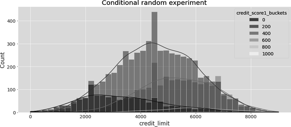
Beta Sampling

In this experiment, credit limit was sampled from Beta distributions. The Beta distribution can be understood as generalization of the uniform distribution, which makes it particularly handy when you want your sample to be confined to a specific range.

This doesn’t mean that conditionally random experiments are better than completely random experiments. They sure are cheaper, but they add a tone of extra complexity. For this reason, if you opt for a conditionally random experiment, for whatever reason, try to keep it as close to a completely random experiment as possible. This means that:

• The lower the number of groups, the easier it will be to deal with the conditionally random test. In this example you only have 5 groups, since you divided credit_score1 in buckets of 200 and the score goes from 0 to 1,000. Combining different groups with different treatment distribution increases the complexity, so sticking to fewer groups is a good idea.

• The bigger the overlap in the treatment distributions across groups, the easier your life will be. This has to do with the positivity assumption. In this example, if the high-risk group had zero probability of receiving high lines, you would have to rely on dangerous extrapolations to know what would happen if they were to receive those high lines.

If you crank these two rules of thumb to their maximum, you get back a completely random experiment, which means both of them carry a trade-off: the lower the number of groups and the higher the overlap, the easier it will be to read the experiment, but it will also be more expensive, and vice versa.

Note

Stratified experiments can also be used as a tool to minimize variance and to ensure balance between treatment and control on the stratified variables. But in those applications, the treatment distribution is designed to be the same across all groups or strata.

Dummy Variables

The neat thing about conditionally random experiments is that the conditional independence assumption is much more plausible, since you know lines were randomly assigned given a categorical variable of your choice. The downside is that a simple regression of the outcome on the treated will yield a biased estimate. For example, here is what happens when you estimate the model, without the confounder included:

$${\mathit{default}}_i={\beta }_0+{\beta }_1{\mathrm{lines}}_i+e_i$$

In [20]: model = smf.ols("default ~ credit_limit", data=risk_data_rnd).fit()
         model.summary().tables[1]
         

	coef	std err	t	P>|t|	[0.025	0.975]
Intercept	0.1369	0.009	15.081	0.000	0.119	0.155
credit_limit	–9.344e–06	1.85e–06	–5.048	0.000	–1.3e–05	–5.72e–06

As you can see, the causal parameter estimate, $\widehat{{\beta }_1}$, is negative, which makes no sense here. Higher credit lines probably do not decrease a customer’s risk. What happened is that, in this data, due to the way the experiment was designed, lower-risk customers—those with high credit_score1—got, on average, higher lines.

To adjust for that, you need to include in the model the group within which the treatment is randomly assigned. In this case, you need to control for credit_score1_buckets. Even though this group is represented as a number, it is actually a categorical variable: it represents a group. So, the way to control for the group itself is to create dummy variables. A dummy is a binary column for a group. It is 1 if the customer belongs to that group and 0 otherwise. As a customer can only be from one group, at most one dummy column will be 1, with all the others being zero. If you come from a machine learning background, you might know this as one-hot encoding. They are exactly the same thing.

In pandas, you can use the pd.get_dummies function to create dummies. Here, I’m passing the column that represents the groups, credit_score1_buckets, and saying that I want to create dummy columns with the suffix sb (for score bucket). Also, I’m dropping the first dummy, that of the bucket 0 to 200. That’s because one of the dummy columns is redundant. If I know that all the other columns are zero, the one that I dropped must be 1:

In [21]: risk_data_dummies = (
	risk_data_rnd
		.join(pd.get_dummies(risk_data_rnd["credit_score1_buckets"],
					prefix="sb",
					drop_first=True))
)
         

	wage	educ	exper	married	...	sb_400	sb_600	sb_800	sb_1000
0	890.0	11	16	1	...	1	0	0	0
1	670.0	11	7	1	...	0	0	0	0
2	1220.0	14	9	1	...	1	0	0	0
3	1210.0	15	8	1	...	0	1	0	0
4	900.0	16	1	1	...	0	0	0	0

Once you have the dummy columns, you can add them to your model and estimate ${\beta }_1$ again:

$${\mathit{default}}_i={\beta }_0+{\beta }_1{\mathrm{lines}}_i+{\theta \mathbf{G}}_i+e_i$$

Now, you’ll get a much more reasonable estimate, which is at least positive, indicating that more credit lines increase risk of default.

In [22]: model = smf.ols(
             "default ~ credit_limit + sb_200+sb_400+sb_600+sb_800+sb_1000",
             data=risk_data_dummies
         ).fit()

         model.summary().tables[1]
         

	coef	std err	t	P>|t|	[0.025	0.975]
Intercept	0.2253	0.056	4.000	0.000	0.115	0.336
credit_limit	4.652e–06	2.02e–06	2.305	0.021	6.97e–07	8.61e–06
sb_200	–0.0559	0.057	–0.981	0.327	–0.168	0.056
sb_400	–0.1442	0.057	–2.538	0.011	–0.256	–0.033
sb_600	–0.2148	0.057	–3.756	0.000	–0.327	–0.103
sb_800	–0.2489	0.060	–4.181	0.000	–0.366	–0.132
sb_1000	–0.2541	0.094	–2.715	0.007	–0.438	–0.071

I’m only showing you how to create dummies by hand so you know what happens under the hood. This will be very useful if you have to implement that sort of regression in some other framework that is not in Python. In Python, if you are using statsmodels, the C() function in the formula can do all of that for you:

In [23]: model = smf.ols("default ~ credit_limit + C(credit_score1_buckets)",
                         data=risk_data_rnd).fit()

         model.summary().tables[1]
         

	coef	std err	t	P>|t|	[0.025	0.975]
Intercept	0.2253	0.056	4.000	0.000	0.115	0.336
C(credit_score1_buckets)[T.200]	–0.0559	0.057	–0.981	0.327	–0.168	0.056
C(credit_score1_buckets)[T.400]	–0.1442	0.057	–2.538	0.011	–0.256	–0.033
C(credit_score1_buckets)[T.600]	–0.2148	0.057	–3.756	0.000	–0.327	–0.103
C(credit_score1_buckets)[T.800]	–0.2489	0.060	–4.181	0.000	–0.366	–0.132
C(credit_score1_buckets)[T.1000]	–0.2541	0.094	–2.715	0.007	–0.438	–0.071
credit_limit	4.652e–06	2.02e–06	2.305	0.021	6.97e–07	8.61e–06

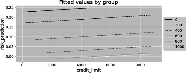
Finally, here you only have one slope parameter. Adding dummies to control for confounding gives one intercept per group, but the same slope for all groups. We’ll discuss this shortly, but this slope will be a variance weighted average of the regression in each group. If you plot the model’s predictions for each group, you can clearly see that you have one line per group, but all of them have the same slope:

Saturated Regression Model

Remember how I started the chapter highlighting the similarities between regression and a conditional average? I showed you how running a regression with a binary treatment is exactly the same as comparing the average between treated and control group. Now, since dummies are binary columns, the parallel also applies here. If you take your conditionally random experiment data and give it to someone that is not as versed in regression as you are, their first instinct will probably be to simply segment the data by credit_score1_buckets and estimate the effect in each group separately:

In [24]: def regress(df, t, y):
             return smf.ols(f"{y}~{t}", data=df).fit().params[t]

         effect_by_group = (risk_data_rnd
                            .groupby("credit_score1_buckets")
                            .apply(regress, y="default", t="credit_limit"))
         effect_by_group
         

Out[24]: credit_score1_buckets
         0      -0.000071
         200     0.000007
         400     0.000005
         600     0.000003
         800     0.000002
         1000    0.000000
         dtype: float64
         

This would give an effect by group, which means you also have to decide how to average them out. A natural choice would be a weighted average, where the weights are the size of each group:

In [25]: group_size = risk_data_rnd.groupby("credit_score1_buckets").size()
         ate = (effect_by_group * group_size).sum() / group_size.sum()
         ate
         

Out[25]: 4.490445628748722e-06
         

Of course, you can do the exact same thing with regression, by running what is called a saturated model. You can interact the dummies with the treatment to get an effect for each dummy defined group. In this case, because the first dummy is removed, the parameter associated with credit_limit actually represents the effect in the omitted dummy group, sb_100. It is the exact same number as the one estimated above for the credit_score1_bucketsearlier group 0 to 200: –0.000071:

In [26]: model = smf.ols("default ~ credit_limit * C(credit_score1_buckets)",
                         data=risk_data_rnd).fit()
         model.summary().tables[1]
         

	coef	std err	t	P>|t|	[0.025	0.975]
Intercept	0.3137	0.077	4.086	0.000	0.163	0.464
C(credit_score1_buckets)[T.200]	–0.1521	0.079	–1.926	0.054	–0.307	0.003
C(credit_score1_buckets)[T.400]	–0.2339	0.078	–3.005	0.003	–0.386	–0.081
C(credit_score1_buckets)[T.600]	–0.2957	0.080	–3.690	0.000	–0.453	–0.139
C(credit_score1_buckets)[T.800]	–0.3227	0.111	–2.919	0.004	–0.539	–0.106
C(credit_score1_buckets)[T.1000]	–0.3137	0.428	–0.733	0.464	–1.153	0.525
credit_limit	–7.072e–05	4.45e–05	–1.588	0.112	–0.000	1.66e–05
credit_limit:C(credit_score1_buckets)[T.200]	7.769e–05	4.48e–05	1.734	0.083	–1.01e–05	0.000
credit_limit:C(credit_score1_buckets)[T.400]	7.565e–05	4.46e–05	1.696	0.090	–1.18e–05	0.000
credit_limit:C(credit_score1_buckets)[T.600]	7.398e–05	4.47e–05	1.655	0.098	–1.37e–05	0.000
credit_limit:C(credit_score1_buckets)[T.800]	7.286e–05	4.65e–05	1.567	0.117	–1.83e–05	0.000
credit_limit:C(credit_score1_buckets)[T.1000]	7.072e–05	8.05e–05	0.878	0.380	–8.71e–05	0.000

The interaction parameters are interpreted in relation to the effect in the first (omitted) group. So, if you sum the parameter associated with credit_limit with other interaction terms, you can see the effects for each group estimated with regression. They are exactly the same as estimating one effect per group:

In [27]: (model.params[model.params.index.str.contains("credit_limit:")]
          + model.params["credit_limit"]).round(9)
         

Out[27]: credit_limit:C(credit_score1_buckets)[T.200]     0.000007
         credit_limit:C(credit_score1_buckets)[T.400]     0.000005
         credit_limit:C(credit_score1_buckets)[T.600]     0.000003
         credit_limit:C(credit_score1_buckets)[T.800]     0.000002
         credit_limit:C(credit_score1_buckets)[T.1000]    0.000000
         dtype: float64
         

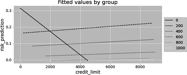
Plotting this model’s prediction by group will also show that, now, it is as if you are fitting a separate regression for each group. Each line will have not only a different intercept, but also a different slope. Besides, the saturated model has more parameters (degrees of freedom), which also means more variance, all else equal. If you look at the following plot, you’ll see a line with negative slope, which doesn’t make sense in this context. However, that slope is not statistically significant. It is probably just noise due to a small sample in that group:

Regression as Variance Weighted Average

But if both the saturated regression and calculating the effect by group give you the exact same thing, there is a very important question you might be asking yourself. When you run the model default ~ credit_limit + C(credit_score1_buckets), without the interaction term, you get a single effect: only one slope parameter. Importantly, if you look back, that effect estimate is different from the one you got by estimating an effect per group and averaging the results using the group size as weights. So, somehow, regression is combining the effects from different groups. And the way it does it is not a sample size weighted average. So what is it then?

Again, the best way to answer this question is by using some very illustrative simulated data. Here, let’s simulate data from two different groups. Group 1 has a size of 1,000 and an average treatment effect of 1. Group 2 has a size of 500 and an average treatment effect of 2. Additionally, the standard deviation of the treatment in group 1 is 1 and 2 in group 2:

In [28]: np.random.seed(123)

         # std(t)=1
         t1 = np.random.normal(0, 1, size=1000)
         df1 = pd.DataFrame(dict(
             t=t1,
             y=1*t1, # ATE of 1
             g=1,
         ))

         # std(t)=2
         t2 = np.random.normal(0, 2, size=500)
         df2 = pd.DataFrame(dict(
             t=t2,
             y=2*t2, # ATE of 2
             g=2,
         ))

         df = pd.concat([df1, df2])
         df.head()
         

	t	y	g
0	–1.085631	–1.085631	1
1	0.997345	0.997345	1
2	0.282978	0.282978	1
3	–1.506295	–1.506295	1
4	–0.578600	–0.578600	1

If you estimate the effects for each group separately and average the results with the group size as weights, you’d get an ATE of around 1.33, $(1*1000+2*500)/1500$:

In [29]: effect_by_group = df.groupby("g").apply(regress, y="y", t="t")
         ate = (effect_by_group *
                df.groupby("g").size()).sum() / df.groupby("g").size().sum()
         ate
         

Out[29]: 1.333333333333333
         

But if you run a regression of y on t while controlling for the group, you get a very different result. Now, the combined effect is closer to the effect of group 2, even though group 2 has half the sample of group 1:

In [30]: model = smf.ols("y ~ t + C(g)", data=df).fit()
         model.params
         

Out[30]: Intercept    0.024758
         C(g)[T.2]    0.019860
         t            1.625775
         dtype: float64
         

The reason for this is that regression doesn’t combine the group effects by using the sample size as weights. Instead, it uses weights that are proportional to the variance of the treatment in each group. Regression prefers groups where the treatment varies a lot. This might seem odd at first, but if you think about it, it makes a lot of sense. If the treatment doesn’t change much within a group, how can you be sure of its effect? If the treatment changes a lot, its impact on the outcome will be more evident.

To summarize, if you have multiple groups where the treatment is randomized inside each group, the conditionality principle states that the effect is a weighted average of the effect inside each group:

$$ATE=E\left\{\left(\frac{\partial }{\partial t}E\left[Y_i\right|T=t,Grou{p}_i]\right)w\left(Grou{p}_i\right)\right\}$$

Depending on the method, you will have different weights. With regression, $w\left(Grou{p}_i\right)\propto {\sigma }^2\left(T\right)|Group$, but you can also choose to manually weight the group effects using the sample size as the weight: $w\left(Grou{p}_i\right)=N_{Group}$.

See Also

Knowing this difference is key to understanding what is going on behind the curtains with regression. The fact that regression weights the group effects by variance is something that even the best researchers need to be constantly reminded of. In 2020, the econometric field went through a renaissance regarding the diff-in-diff method (you’ll see more about it in Part IV). At the center of the issue was regression not weighting effects by sample size. If you want to learn more about it, I recommend checking it out the paper “Difference-in-Differences with Variation in Treatment Timing,” by Andrew Goodman-Bacon. Or just wait until we get to Part IV.

De-Meaning and Fixed Effects

You just saw how to include dummy variables in your model to account for different treatment assignments across groups. But it is with dummies where the FWL theorem really shines. If you have a ton of groups, adding one dummy for each is not only tedious, but also computationally expensive. You would be creating lots and lots of columns that are mostly zero. You can solve this easily by applying FWL and understanding how regression orthogonalizes the treatment when it comes to dummies.

You already know that the debiasing step in FWL involves predicting the treatment from the covariates, in this case, the dummies:

In [31]: model_deb = smf.ols("credit_limit ~ C(credit_score1_buckets)",
                             data=risk_data_rnd).fit()
         model_deb.summary().tables[1]
         

	coef	std err	t	P>|t|	[0.025	0.975]
Intercept	1173.0769	278.994	4.205	0.000	626.193	1719.961
C(credit_score1_buckets)[T.200]	2195.4337	281.554	7.798	0.000	1643.530	2747.337
C(credit_score1_buckets)[T.400]	3402.3796	279.642	12.167	0.000	2854.224	3950.535
C(credit_score1_buckets)[T.600]	4191.3235	280.345	14.951	0.000	3641.790	4740.857
C(credit_score1_buckets)[T.800]	4639.5105	291.400	15.921	0.000	4068.309	5210.712
C(credit_score1_buckets)[T.1000]	5006.9231	461.255	10.855	0.000	4102.771	5911.076

Since dummies work basically as group averages, you can see that, with this model, you are predicting exactly that: if credit_score1_buckets=0, you are predicting the average line for the group credit_score1_buckets=0; if credit_score1_buckets=1, you are predicting the average line for the group credit_score1_buckets=1 (which is given by summing the intercept to the coefficient for that group $1173.0769+2195.4337=3368.510638$) and so on and so forth. Those are exactly the group averages:

In [32]: risk_data_rnd.groupby("credit_score1_buckets")["credit_limit"].mean()
         

Out[32]: credit_score1_buckets
         0       1173.076923
         200     3368.510638
         400     4575.456498
         600     5364.400448
         800     5812.587413
         1000    6180.000000
         Name: credit_limit, dtype: float64
         

Which means that if you want to residualize the treatment, you can do that in a much simpler and effective way. First, calculate the average treatment for each group:

In [33]: risk_data_fe = risk_data_rnd.assign(
             credit_limit_avg = lambda d: (d
                                           .groupby("credit_score1_buckets")
                                           ["credit_limit"].transform("mean"))
         )
         

Then, to get the residuals, subtract that group average from the treatment. Since this approach subtracts the average treatment, it is sometimes referred to as de-meaning the treatment. If you want to do that inside the regression formula, you must wrap the mathematical operation around I(...):

In [34]: model = smf.ols("default ~ I(credit_limit-credit_limit_avg)",
                         data=risk_data_fe).fit()
         model.summary().tables[1]
         

	coef	std err	t	P>|t|	[0.025	0.975]
Intercept	0.0935	0.003	32.121	0.000	0.088	0.099
I(credit_limit – credit_limit_avg)	4.652e–06	2.05e–06	2.273	0.023	6.4e–07	8.66e–06

The parameter estimate you got here is exactly the same as the one you got when adding dummies to your model. That’s because, mathematically speaking, they are equivalent. This idea goes by the name of fixed effects, since you are controlling for anything that is fixed within a group. It comes from the literature of causal inference with temporal structures (panel data), which you’ll explore more in Part IV.

Another idea from the same literature is to include the average treatment by group in the regression model (from Mundlak’s, 1978). Regression will residualize the treatment from the additional variables included, so the effect here is about the same:

In [35]: model = smf.ols("default ~ credit_limit + credit_limit_avg",
                         data=risk_data_fe).fit()
         model.summary().tables[1]
         

	coef	std err	t	P>|t|	[0.025	0.975]
Intercept	0.4325	0.020	21.418	0.000	0.393	0.472
credit_limit	4.652e–06	2.02e–06	2.305	0.021	6.96e–07	8.61e–06
credit_limit_avg	-7.763e–05	4.75e–06	–16.334	0.000	–8.69e–05	–6.83e–05

Marketing Mix Modeling

Measuring the impact of advertising on sales is very hard, since you usually can’t randomize who gets to see your ads. One popular alternative to randomization in the advertising industry is the technique called marketing mix modeling (MMM). Despite the fancy name, MMMs are just regressions of sales on marketing strategies indicators and some confounders. For example, let’s say you want to know the effect of your budget on TV, social media, and search advertising on your product’s sales. You can run a regression model where each unit $i$ is a day:

$$\begin{array}{c}\hfill \begin{array}{cc}\hfill Sale{s}_i& ={\delta }_0+{\beta }_{1}T{V}_i+{\beta }_{2}Socia{l}_i+{\beta }_{3}Searc{h}_i\hfill \\ & +{\delta }_{1}CompetitorSale{s}_i+{\delta }_{2}Mont{h}_i+{\delta }_{3}Tren{d}_i+e_i\hfill \end{array}\end{array}$$

To account for the fact that you might have increased your marketing budget on a good month, you can adjust for this confounder by including additional controls in your regression. For example, you can include your competitor’s sales, a dummy for each month, and a trend variable.

Omitted Variable Bias: Confounding Through the Lens of Regression

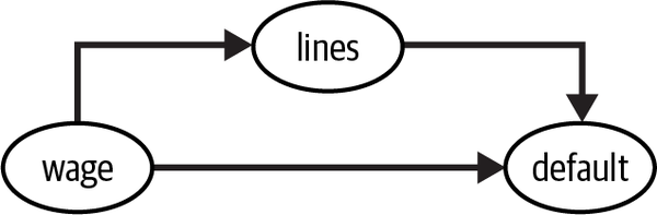
I hope I made myself very clear in Chapter 3 when I said that common causes—confounders—will bias the estimated relationship between the treated and the outcome. That is why you need to account for them by, for example, including them in a regression model. However, regression has its own particular take on confounding bias. Sure, everything said up until now still holds. But regression allows you to be more precise about the confounding bias. For example, let’s say you want to estimate the effect of credit lines on default and that wage is the only confounder:

In this case, you know you should be estimating the model that includes the confounder:

$${\mathit{default}}_i={\beta }_0+{\beta }_1{\mathrm{lines}}_i+{\beta }_2>{\mathrm{wage}}_i+e_i,$$

But if you instead estimate a shorter model, where the confounder is omitted:

$${\mathit{default}}_i={\beta }_0+{\beta }_1{\mathrm{lines}}_i+e_i,$$

the resulting estimate becomes biased:

In [36]: short_model = smf.ols("default ~ credit_limit", data=risk_data).fit()
         short_model.params["credit_limit"]
         

Out[36]: -2.401961992596885e-05
         

As you can see, it looks like higher credit lines cause default to go down, which is nonsense. But you know that already. What you don’t know is that you can be precise about the size of that bias. With regression, you can say that the bias due to an omitted variable is equal to the effect in the model where it is included plus the effect of the omitted variable on the outcome times the regression of omitted on included. Don’t worry. I know this is a mouthful, so let’s digest it little by little. First, it means that simple regression of $Y$ on $T$ will be the true causal parameter $\tau$, plus a bias term:

$${\displaystyle \frac{Cov(T,Y)}{Var\left(T\right)}}=\tau +{\beta }_{omitted}^{\text{'}}{\delta }_{omitted}$$

This bias term is the coefficient of the omitted confounder on the outcome, ${\beta }_{omitted}$, times the coefficient of regressing the omitted variable on the treatment, ${\delta }_{omitted}$. To check that, you can obtain the biased parameter estimate you got earlier with the following code, which reproduces the omitted variable bias formula:

In [37]: long_model = smf.ols("default ~ credit_limit + wage",
                              data=risk_data).fit()

         omitted_model = smf.ols("wage ~ credit_limit", data=risk_data).fit()

         (long_model.params["credit_limit"] 
          + long_model.params["wage"]*omitted_model.params["credit_limit"])
         

Out[37]: -2.4019619925968762e-05
         

Neutral Controls

By now, you probably have a good idea about how regression adjusts for confounder variables. If you want to know the effect of the treatment $T$ on $Y$ while adjusting for confounders $X$, all you have to do is include $X$ in the model. Alternatively, to get the exact same result, you can predict $T$ from $X$, get the residuals, and use that as a debiased version of the treatment. Regressing $Y$ on those residuals will give you the relationship of $T$ and $Y$ while holding $X$ fixed.

But what kind of variables should you include in $X$? Again, it’s not because adding variables adjusts for them that you want to include everything in your regression model. As seen in the previous chapters, you don’t want to include common effects (colliders) or mediators, as those would induce selection bias. But in the context of regression, there are more types of controls you should know about. Controls that, at first, seem like they are innocuous, but are actually quite harmful. These controls are named neutral because they don’t influence the bias in your regression estimate. But they can have severe implications in terms of variance. As you’ll see, there is a bias–variance trade-off when it comes to including certain variables in your regression. Consider, for instance, the following DAG:

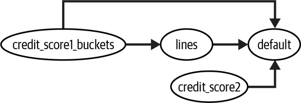
Should you include credit_score2 in your model? If you don’t include it, you’ll get the same result you’ve been seeing all along. That result is unbiased, as you are adjusting for credit_score1_buckets. But, although you don’t need to, look at what happens when you do include credit_score2. Compare the following results to the one you got earlier, which didn’t include credit_score2. What changed?

In [38]: formula = "default~credit_limit+C(credit_score1_buckets)+credit_score2"
         model = smf.ols(formula, data=risk_data_rnd).fit()
         model.summary().tables[1]
         

	coef	std err	t	P>|t|	[0.025	0.975]
Intercept	0.5576	0.055	10.132	0.000	0.450	0.665
C(credit_score1_buckets)[T.200]	–0.0387	0.055	–0.710	0.478	–0.146	0.068
C(credit_score1_buckets)[T.400]	–0.1032	0.054	–1.898	0.058	–0.210	0.003
C(credit_score1_buckets)[T.600]	–0.1410	0.055	–2.574	0.010	–0.248	–0.034
C(credit_score1_buckets)[T.800]	–0.1161	0.057	–2.031	0.042	–0.228	–0.004
C(credit_score1_buckets)[T.1000]	–0.0430	0.090	–0.479	0.632	–0.219	0.133
credit_limit	4.928e–06	1.93e–06	2.551	0.011	1.14e–06	8.71e–06
credit_score2	–0.0007	2.34e–05	–30.225	0.000	–0.001	–0.001

First, the parameter estimate on credit_limit became a bit higher. But, more importantly, the standard error decreases. That’s because credit_score2 is a good predictor of the outcome $Y$ and it will contribute to the denoising step of linear regression. In the final step of FWL, because credit_score2 was included, the variance in $\tilde{Y}$ will be reduced, and regressing it on $\tilde{T}$ will yield more precise results.

This is a very interesting property of linear regression. It shows that it can be used not only to adjust for confounders, but also to reduce noise. For example, if you have data from a properly randomized A/B test, you don’t need to worry about bias. But you can still use regression as a noise reduction tool. Just include variables that are highly predictive of the outcome (and that don’t induce selection bias).

Noise Reduction Techniques

There are other noise reduction techniques out there. The most famous one is CUPED, which was developed by Microsoft researchers and is widely used in tech companies. CUPED is very similar to just doing the denoising part of the FWL theorem.

Noise Inducing Control

Just like controls can reduce noise, they can also increase it. For example, consider again the case of a conditionally random experiment. But this time, you are interested in the effect of credit limit on spend, rather than on risk. Just like in the previous example, credit limit was randomly assigned, given credit_score1. But this time, let’s say that credit_score1 is not a confounder. It causes the treatment, but not the outcome. The causal graph for this data-generating process looks like this:

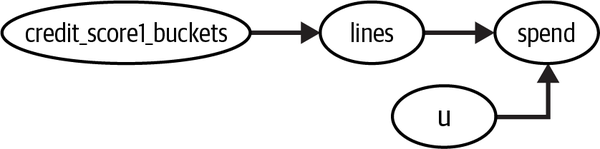
This means that you don’t need to adjust for credit_score1 to get the causal effect of credit limit on spend. A single variable regression model would do. Here, I’m keeping the square root function to account for the concavity in the treatment response function:

In [39]: spend_data_rnd = pd.read_csv("data/spend_data_rnd.csv")

         model = smf.ols("spend ~ np.sqrt(credit_limit)",
                         data=spend_data_rnd).fit()

         model.summary().tables[1]
         

	coef	std err	t	P>|t|	[0.025	0.975]
Intercept	2153.2154	218.600	9.850	0.000	1723.723	2582.708
np.sqrt(credit_limit)	16.2915	2.988	5.452	0.000	10.420	22.163

But, what happens if you do include credit_score1_buckets?

In [40]: model = smf.ols("spend~np.sqrt(credit_limit)+C(credit_score1_buckets)",
                         data=spend_data_rnd).fit()

         model.summary().tables[1]
         

	coef	std err	t	P>|t|	[0.025	0.975]
Intercept	2367.4867	556.273	4.256	0.000	1274.528	3460.446
C(credit_score1_buckets)[T.200]	–144.7921	591.613	–0.245	0.807	–1307.185	1017.601
C(credit_score1_buckets)[T.400]	–118.3923	565.364	–0.209	0.834	–1229.211	992.427
C(credit_score1_buckets)[T.600]	–111.5738	570.471	–0.196	0.845	–1232.429	1009.281
C(credit_score1_buckets)[T.800]	–89.7366	574.645	–0.156	0.876	–1218.791	1039.318
C(credit_score1_buckets)[T.1000]	363.8990	608.014	0.599	0.550	–830.720	1558.518
np.sqrt(credit_limit)	14.5953	3.523	4.142	0.000	7.673	21.518

You can see that it increases the standard error, widening the confidence interval of the causal parameter. That is because, like you saw in “Regression as Variance Weighted Average”, OLS likes when the treatment has a high variance. But if you control for a covariate that explains the treatment, you are effectively reducing its variance.

Feature Selection: A Bias-Variance Trade-Off

In reality, it’s really hard to have a situation where a covariate causes the treatment but not the outcome. Most likely, you will have a bunch of confounders that cause both $T$ and $Y$, but to different degrees. In Figure 4-3, $X_1$ is a strong cause of $T$ but a weak cause of $Y$, $X_3$ is a strong cause of $Y$ but a weak cause of $T$, and $X_2$ is somewhere in the middle, as denoted by the thickness of each arrow.

Figure 4-3. A confounder like $X_1$, which explains away the variance in the treatment more than it removes bias, might be causing more harm than good to your estimator

In these situations, you can quickly be caught between a rock and a hard place. On one hand, if you want to get rid of all the biases, you must include all the covariates; after all, they are confounders that need to be adjusted. On the other hand, adjusting for causes of the treatment will increase the variance of your estimator.

To see that, let’s simulate data according to the causal graph in Figure 4-3. Here, the true ATE is 0.5. If you try to estimate this effect while controlling for all of the confounders, the standard error of your estimate will be too high to conclude anything:

In [41]: np.random.seed(123)

         n = 100
         (x1, x2, x3) = (np.random.normal(0, 1, n) for _ in range(3))
         t = np.random.normal(10*x1 + 5*x2 + x3)

         # ate = 0.05
         y = np.random.normal(0.05*t + x1 + 5*x2 + 10*x3, 5)
         df = pd.DataFrame(dict(y=y, t=t, x1=x1, x2=x2, x3=x3))

         smf.ols("y~t+x1+x2+x3", data=df).fit().summary().tables[1]
         

	coef	std err	t	P>|t|	[0.025	0.975]
Intercept	0.2707	0.527	0.514	0.608	–0.775	1.316
t	0.8664	0.607	1.427	0.157	–0.339	2.072
x1	–7.0628	6.038	–1.170	0.245	–19.049	4.923
x2	0.0143	3.128	0.005	0.996	–6.195	6.224
x3	9.6292	0.887	10.861	0.000	7.869	11.389

If you know that one of the confounders is a strong predictor of the treatment and a weak predictor of the outcome, you can choose to drop it from the model. In this example, that would be $X_1$. Now, be warned! This will bias your estimate. But maybe this is a price worth paying if it also decreases variance significantly:

In [42]: smf.ols("y~t+x2+x3", data=df).fit().summary().tables[1]
         

	coef	std err	t	P>|t|	[0.025	0.975]
Intercept	0.1889	0.523	0.361	0.719	–0.849	1.227
t	0.1585	0.046	3.410	0.001	0.066	0.251
x2	3.6095	0.582	6.197	0.000	2.453	4.766
x3	10.4549	0.537	19.453	0.000	9.388	11.522

The bottom line is that the more confounders you include (adjust for) in your model, the lower the bias in your causal estimate. However, if you include variables that are weak predictors of the outcome but strong predictors of the treatment, this bias reduction will come at a steep cost in terms of variance increase. Saying the same thing but differently, sometimes it is worth accepting a bit of bias in order to reduce variance. Also, you should be very aware that not all confounders are equal. Sure, all of them are common because of both $T$ and $Y$. But if they explain the treatment too much and almost nothing about the outcome, you should really consider dropping it from your adjustment. This is valid for regression, but it will also be true for other adjustment strategies, like propensity score weighting (see Chapter 5).

Unfortunately, how weak the confounder should be in terms of explaining the treatment to justify removing it is still an open question in causal inference. Still, it is worth knowing that this bias-variance trade-off exists, as it will help you understand and explain what is going on with your linear regression.

Key Ideas

This chapter was about regression, but from a very different perspective than the one you usually see in machine learning books. Regression here is not a prediction tool. Notice how I didn’t talk about $R^2$ even once! Rather, regression is used here as a way to primarily adjust for confounders and, sometimes, as a variance reduction technique.

The core of this chapter was orthogonalization as a means to make treatment look as good as randomly assigned if conditional independence holds. Formally, if $Y_t\perp T|X$, you can adjust for the confounding bias due to $X$ by regressing $T$ on $X$ and obtaining the residuals. Those residuals can be seen as a debiased version of the treatment.

This approach was further developed using the Frisch-Waugh-Lovell theorem, which states that a multivariate regression can be decomposed into the following steps:

1. A debiasing step, where you regress the treatment $T$ on confounders $X$ and obtain the treatment residuals $\tilde{T}=T-\widehat{T}$

2. A denoising step, where you regress the outcome $Y$ on the confounder variables $X$ and obtain the outcome residuals $\tilde{Y}=Y-\widehat{Y}$

3. An outcome model where you regress the outcome residual $\tilde{Y}$ on the treatment residual $\tilde{T}$ to obtain an estimate for the causal effect of $T$ on $Y$

Everything else in the chapter follows from this theorem—be it nonlinear treatment response functions, understanding how regression with categorical variables implements a weighted average, or the role of good and bad controls in regression.