Causal Inference in Python

Chapter 1. Introduction to Causal Inference

In this first chapter I’ll introduce you to a lot of the fundamental concepts of causal inference as well as its main challenges and uses. Here, you will learn a lot of jargon that will be used in the rest of the book. Also, I want you to always keep in mind why you need causal inference and what you can do with it. This chapter will not be about coding, but about very important first concepts of causal inference.

What Is Causal Inference?

Causality is something you might know as a dangerous epistemological terrain you must avoid going into. Your statistics teacher might have said over and over again that “association is not causation” and that confusing the two would cast you to academic ostracism or, at the very least, be severely frowned upon. But you see, that is the thing: sometimes, association is causation.

We humans know this all too well, since, apparently, we’ve been primed to take association for causation. When you decide not to drink that fourth glass of wine, you correctly inferred that it would mess you up on the next day. You are drawing from past experience: from nights when you drank too much and woke up with a headache; from nights you took just one glass of wine, or none at all, and nothing happened. You’ve learned that there is something more to the association between drinking and hangovers. You’ve inferred causality out of it.

On the flip side, there is some truth to your stats teacher’s warnings. Causation is a slippery thing. When I was a kid, I ate calamari doré twice and both times it ended terribly, which led me to conclude I was allergic to squid (and clam, octopus, and any other type of sea invertebrate). It took me more than 20 years to try it again. When I did, it was not only delicious, but it also caused me no harm. In this case, I had confused association with causation. This was a harmless confusion, as it only deprived me of delicious seafood for some years, but mistaking association for causation can have much more severe consequences. If you invest in the stock market, you’ve probably been through a situation where you decided to put money in just before a steep increase in prices, or to withdraw just before everything collapsed. This likely tempted you to think you could time the market. If you managed to ignore that temptation, good for you. But many fall for it, thinking that their intuition is causally linked to the erratic movements of stocks. In some situations, this belief leads to riskier and riskier bets until, eventually, almost everything is lost.

In a nutshell, association is when two quantities or random variables move together, whereas causality is when change in one variable causes change in another. For example, you could associate the number of Nobel Prizes a country has with the per-capita consumption of chocolate, but even though these variables might move together, it would be foolish to think one causes the other. It’s easy to see why association doesn’t imply causation, but equating the two is a whole different matter. Causal inference is the science of inferring causation from association and understanding when and why they differ.

Why We Do Causal Inference

Causal inference can be done for the sole purpose of understanding reality. But there is often a normative component to it. The reason you’ve inferred that too much drinking causes headaches is that you want to change your drinking habits to avoid the pain. The company you work for wants to know if marketing costs cause growth in revenues because, if they do, managers can use it as a leverage to increase profits. Generally speaking, you want to know cause-and-effect relationships so that you can intervene on the cause to bring upon a desired effect. If you take causal inference to the industry, it becomes mostly a branch of the decision-making sciences.

Since this book is mostly industry focused, it will cover the part of causal inference that is preoccupied with understanding the impact of interventions. What would happen if you used another price instead of this price you’re currently asking for your merchandise? What would happen if you switch from this low-sugar diet you’re on to that low-fat diet? What will happen to the bank’s margins if it increases the customers’ credit line? Should the government give tablets to every kid in school to boost their reading test score or should it build an old-fashioned library? Is marrying good for your personal finances or are married couples wealthier just because wealthy people are more likely to attract a partner in the first place? These questions are all practical. They stem from a desire to change something in your business or in your life so that you can be better off.

Machine Learning and Causal Inference

If you take a deeper look at the types of questions you want to answer with causal inference, you will see they are mostly of the “what if” type. I’m sorry to be the one that says it, but machine learning (ML) is just awful at those types of questions.

ML is very good at answering prediction questions. As Ajay Agrawal, Joshua Gans, and Avi Goldfarb put it in the book Prediction Machines (Harvard Business Review Press), “the new wave of artificial intelligence does not actually bring us intelligence but instead a critical component of intelligence—prediction.” You can do all sorts of beautiful things with machine learning. The only requirement is to frame your problems as prediction ones. Want to translate from English to Portuguese? Then build an ML model that predicts Portuguese sentences when given English sentences. Want to recognize faces? Then create an ML model that predicts the presence of a face in a subsection of a picture.

However, ML is not a panacea. It can perform wonders under rigid boundaries and still fail miserably if its data deviates a little from what the model is accustomed to. To give another example from Prediction Machines, “in many industries, low prices are associated with low sales. For example, in the hotel industry, prices are low outside the tourist season, and prices are high when demand is highest and hotels are full. Given that data, a naive prediction might suggest that increasing the price would lead to more rooms sold.”

Machine learning uses associations between variables to predict one from the other. It will work incredibly well as long as you don’t change the variables it is using to make predictions. This completely defeats the purpose of using predictive ML for most decision making that involves interventions.

The fact that most data scientists know a lot of ML but not much about causal inference leads to an abundance of ML models being deployed where they are not useful for the task at hand. One of the main goals of companies is to increase sales or usage. Yet, an ML model that just predicts sales is oftentimes useless—if not harmful—for this purpose. This model might even conclude something nonsensical, as in the example where high volumes of sales are associated with high prices. Yet, you’d be surprised by how many companies implement predictive ML models when the goal they have in mind has nothing to do with predictions.

This does not mean that ML is completely useless for causal inference. It just means that, when naively applied, it often does more harm than good. But if you approach ML from a different angle, as a toolbox of powerful models rather than purely predictive machines, you’ll start to see how they can connect to the goals of causal inference. In Part III I’ll show what you need to watch out for when mixing ML and causal inference and how to repurpose common ML algorithms, like decision trees and gradient boosting, to do causal inference.

Association and Causation

Intuitively, you kind of know why association is not causation. If someone tells you that top-notch consulting causes your business to improve, you are bound to raise an eyebrow. How can you know if the consulting firm is actually causing business to improve or if it is just that only flourishing businesses have the luxury to hire those services?

To make things a bit more tangible, put yourself in the shoes of an online marketplace company. Small and medium-sized businesses use your online platform to advertise and sell their products. These businesses have complete autonomy in stuff like setting prices and when to have sales. But it is in the best interest of your company that these businesses flourish and prosper. So, you decide to help them by giving guidance on how, if, and when to set up a sales campaign where they announce a temporary price drop to consumers. To do that, the first thing you need to know is the impact of lowering prices on units sold. If the gains from selling more compensate for the loss of selling cheaper, sales will be a good idea. If you hadn’t already noticed, this is a causal question. You need to answer how many additional units a business would have sold had they lowered prices compared to not doing anything.

Needless to say, this is a complicated question; maybe too complicated for the beginning of this book. Different businesses operate within your platform. Some sell food; some sell clothes. Some sell fertilizers and agricultural products. As a result, price cuts might have different impacts depending on the type of business. For instance, it might be a good idea for a clothing business to announce lower prices one week prior to Father’s Day. Yet, a similar price drop for an agribusiness will probably do very little. So, let’s simplify the problem a bit. Let’s focus your attention on only one type of business: those that sell kids’ toys. Also, let’s focus your attention on one period of the year: December, before Christmas. For now, you’ll just try to answer how cutting prices during these periods increases sales so you can pass this information along to the businesses operating in the kids’ toy industry, allowing them to make better decisions.

To decide if sales is a good idea, you can leverage information from multiple kids’ toys businesses. This data is stored in a pandas data frame for you to access. Here are the first few rows for you to get a sense of what you are dealing with:

	store	weeks_to_xmas	avg_week_sales	is_on_sale	weekly_amount_sold
0	1	3	12.98	1	219.60
1	1	2	12.98	1	184.70
2	1	1	12.98	1	145.75
3	1	0	12.98	0	102.45
4	2	3	19.92	0	103.22
5	2	2	19.92	0	53.73

The first column is the store’s unique identifier (ID). You have weekly data for each store in the month of December. You also have information about the size of each business in terms of average products sold per week during that year. A boolean column (0 or 1) flags the business as having a sale at the time. The last column shows the average weekly sales of that store during that week.

Unit of Analysis

The unit of analysis in a causal inference study is usually the thing you wish to intervene on (treat). In most cases, the unit of analysis will be people, as when you want to know the effect of a new product on customer retention. But it is not uncommon to have other types of units. For instance, in this chapter’s example, the unit of analysis is business. In this same example, you could also try to answer when is the best moment to have sales, in which case the unit of analysis would be a time period (week, in this case).

The Treatment and the Outcome

Now that you have some data to look at, it’s time to learn our first bit of technicality. Let’s call $T_i$ the treatment for unit i:

$T_i=\left\{\begin{array}{c}1\text{if}\text{unit}\mathit{\text{i}}\text{received}\text{the}\text{treatment}\hfill \\ 0\text{otherwise}\hfill \end{array}\right.$

The treatment here doesn’t need to be medicine or anything from the medical field. Instead, it is just a term I’ll use to denote some intervention for which I want to know the effect of. In this case, the treatment is simply a price drop for one of the businesses inside your online platform, represented by the column is_on_sale.

Treatment Notation

In some texts and later on in this book, you’ll sometimes see $D$ instead of $T$ to denote the treatment. $D$ will avoid much confusion when you have a time dimension to your causal problems.

Additionally, I’ll be referring to weekly_amount_sold (the variable that I want to influence here) as the outcome. I’ll represent the outcome for unit $i$ with $Y_i$. With these two new concepts, I can restate the goal of causal inference as the process of learning the impact $T$ has on $Y$. In our example, this amounts to figuring out the effect of is_on_sale on weekly_amount_sold.

The Fundamental Problem of Causal Inference

Here is where things get interesting. The fundamental problem of causal inference is that you can never observe the same unit with and without treatment. It is as if you have two diverging roads and can only know what lies ahead of the one taken. To fully appreciate this issue, let’s go back to our example and plot the outcome by the treatment, that is, weekly_amount_sold by is_on_sale. You can immediately see that the stores that dropped their price sell a lot more (see Figure 1-1).

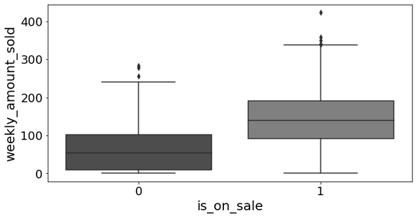
Figure 1-1. Amount sold per week during sales (1) and without sales (0)

This also matches our intuition about how the world works: people buy more when prices are low and sales (usually) means lower prices. This is very nice, as causal inference goes hand in hand with expert knowledge. But you shouldn’t be too careless. It is probably the case that giving and advertising discounts will make customers buy more. But this much more? From the plot in Figure 1-1, it looks like the amount sold is about 150 units higher, on average, when a sale is going on than otherwise. This sounds suspiciously high, since the range of units sold when there is no sale is about 0 to 50. If you scratch your brains a bit, you can start to see that you might be mistaking association for causation. Maybe it is the case that only larger businesses, which are the ones that sell the most anyway, can afford to do aggressive price drops. Maybe businesses have sales closer to Christmas and that’s when customers buy the most anyway.

The point is, you would only be certain about the true effect of price cuts on units sold if you could observe the same business (unit), at the same time, with and without sales going on. Only if you compare these two counterfactual situations will you be sure about the effect of price drops. However, as discussed earlier, the fundamental problem of causal inference is that you simply can’t do that. Instead, you’ll need to come up with something else.

Causal Models

You can reason about all these problems intuitively, but if you want to go beyond simple intuition, you need some formal notation. This will be our everyday language to speak about causality. Think of it as the common tongue we will use with fellow practitioners of the arts of causal inference.

A causal model is a series of assignment mechanisms denoted by $\leftarrow$. In these mechanisms, I’ll use $u$ to denote variables outside the model, meaning I am not making a statement about how they are generated. All the others are variables I care very much about and are hence included in the model. Finally, there are functions $f$ that map one variable to another. Take the following causal model as an example:

$$\begin{array}{c}\hfill T\leftarrow f_t\left(u_t\right)\\ \hfill Y\leftarrow f_y(T,u_y)\end{array}$$

With the first equation, I’m saying that $u_t$, a set of variables I’m not explicitly modeling (also called exogenous variables), causes the treatment $T$ via the function $f_t$. Next, $T$ alongside another set of variables $u_y$ (which I’m also choosing not to model) jointly causes the outcome $Y$ via the function $f_y$. $u_y$ is in this last equation to say that the outcome is not determined by the treatment alone. Some other variables also play a role in it, even if I’m choosing not to model them. Bringing this to the sales example, it would mean that weekly_amount_sold is caused by the treatment is_on_sale and other factors that are not specified, represented as $u$. The point of $u$ is to account for all the variation in the variables caused by it that are not already accounted for by the variables included in the model—also called endogenous variables. In our example, I could say that price drops are caused by factors—could be business size, could be something else—that are not inside the model:

$$\begin{array}{c}\hfill IsOnSales\leftarrow f_t\left(u_t\right)\\ \hfill AmountSold\leftarrow f_y(IsOnSales,u_y)\end{array}$$

I’m using $\leftarrow$ instead of $=$ to explicitly state the nonreversibility of causality. With the equals sign, $Y=T+X$ is equivalent to $T=Y-X$, but I don’t want to say that $T$ causing $Y$ is equivalent to $Y$ causing $T$. Having said that, I’ll often refrain from using $\leftarrow$ just because it’s a bit cumbersome. Just keep in mind that, due to nonreversibility of cause and effects, unlike with traditional algebra, you can’t simply throw things around the equal sign when dealing with causal models.

If you want to explicitly model more variables, you can take them out of $u$ and account for them in the model. For example, remember how I said that the large difference you are seeing between price cuts and no price cuts could be because larger businesses can engage in more aggressive sales? In the previous model, $BusinessSize$ is not explicitly included in the model. Instead, its impact gets relegated to the side, with everything else in $u$. But I could model it explicitly:

$$\begin{array}{c}\hfill BusinessSize\leftarrow f_s\left(u_s\right)\\ \hfill IsOnSales\leftarrow f_t(BusinessSize,u_t)\\ \hfill AmountSold\leftarrow f_y(IsOnSales,BusinessSize,u_y)\end{array}$$

To include this extra endogenous variable, first, I’m adding another equation to represent how that variable came to be. Next, I’m taking $BusinessSize$ out of $u_t$. That is, I’m no longer treating it as a variable outside the model. I’m explicitly saying that $BusinessSize$ causes $IsOnSales$ (along with some other external factors that I’m still choosing not to model). This is just a formal way of encoding the beliefs that bigger businesses are more likely to cut prices. Finally, I can also add $BusinessSize$ to the last equation. This encodes the belief that bigger businesses also sell more. In other words, $BusinessSize$ is a common cause to both the treatment $IsOnSales$ and the outcome $AmountSold$.

Since this way of modeling is probably new to you, it’s useful to link it to something perhaps more familiar. If you come from economics or statistics, you might be used to another way of modeling the same problem:

$$AmountSol{d}_i=\alpha +{\beta }_{1}IsOnSale{s}_i+{\beta }_{2}BusinessSiz{e}_i+e_i$$

It looks very different at first, but closer inspection will reveal how the preceding model is very similar to the one you saw earlier. First, notice how it is just replacing the final equation in that previous model and opening up the $f_y$ function, stating explicitly that endogenous variables $IsOnSales$ and $BusinessSize$ are linearly and additively combined to form the outcome $AmountSold$. In this sense, this linear model assumes more than the one you saw earlier. You can say that it imposes a functional form to how the variables relate to each other. Second, you are not saying anything about how the independent (endogenous) variables—$IsOnSales$ and $BusinessSize$—come to be. Finally, this model uses the equals sign, instead of the assignment operator, but we already agreed not to stress too much about that.

Interventions

The reason I’m taking my time to talk about causal models is because, once you have one, you can start to tinker with it in the hopes of answering a causal question. The formal term for this is intervention. For example, you could take that very simple causal model and force everyone to take the treatment $t_0$. This will eliminate the natural causes of $T$, replacing them by a single constant:

$$\begin{array}{c}\hfill T\leftarrow t_0\\ \hfill Y\leftarrow f_y(T,u_y)\end{array}$$

This is done as a thought experiment to answer the question “what would happen to the outcome $Y$ if I were to set the treatment to $t_0$?” You don’t actually have to intervene on the treatment (although you could and will, but later). In the causal inference literature, you can refer to these interventions with a $do(.)$ operator. If you want to reason about what would happen if you intervene on $T$, you could write $do(T=t_0)$.

Expectations

I’ll use a lot of expectations and conditional expectations from now on. You can think about expectations as the population value that the average is trying to estimate. $E\left[X\right]$ denotes the (marginal) expected values of the random variable X. It can be approximated by the sample average of X. $E\left[Y\right|X=x]$ denotes the expected value of Y when $X=x$. This can be approximated by the average of $Y$ when $X=x$.

The $do(.)$ operator also gives you a first glance at why association is different from causation. I have already argued how high sales volume for a business having a sale, $E\left[AmountSold\right|IsOnSales=1]$, could overestimate the average sales volume a business would have had if it made a price cut, $E\left[AmountSold\right|do(IsOnSales=1)]$. In the first case, you are looking at businesses that chose to cut prices, which are probably bigger businesses. In contrast, the latter quantity, $E\left[AmountSold\right|do(IsOnSales=1)]$, refers to what would’ve happened if you forced every business to engage in sales, not just the big ones. Importantly, in general,

$$E\left[AmountSold\right|IsOnSales=1]\ne E[AmountSold\left|do\right(IsOnSales=1\left)\right]$$

One way to think about the difference between the two is in terms of selection and intervention. When you condition on sales, you are measuring the amount sold on a selected subsample of business that actually cut prices. When you condition on the intervention $do\left(IsOnSales\right)$, you are forcing every business to cut prices and then measuring the amount sold on the entire sample (see Figure 1-2).

$do(.)$ is used to define causal quantities that are not always recoverable from observed data. In the previous example, you can’t observe $do(IsOnSales=1)$ for every business, since you didn’t force them to do sales. $do(.)$ is most useful as a theoretical concept that you can use to explicitly state the causal quantity you are after. Since it is not directly observable, a lot of causal inference is about eliminating it from theoretical expression—a process called identification.

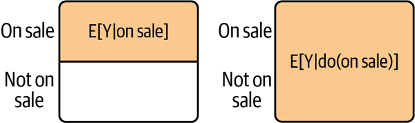
Figure 1-2. Selection filters the sample based on the treatment; intervention forces the treatment on the entire sample

Individual Treatment Effect

The $do(.)$ operator also allows you to express the individual treatment effect, or the impact of the treatment on the outcome for an individual unit $i$. You can write it as the difference between two interventions:

$${\tau }_i=Y_i|do(T=t_1)-Y_i|do(T=t_0)$$

In words, you would read this as “the effect, ${\tau }_i$, of going from treatment $t_0$ to $t_1$ for unit $i$ is the difference in the outcome of that unit under $t_1$ compared to $t_0$”. You could use this to reason about our problem of figuring out the effect of flipping $IsOnSales$ from 0 to 1 in $AmountSold$:

$${\tau }_i=AmountSol{d}_i|do(IsOnSales=1)-AmountSol{d}_i|do(IsOnSales=0)$$

Due to the fundamental problem of causal inference, you can only observe one term of the preceding equation. So, even though you can theoretically express that quantity, it doesn’t necessarily mean you can recover it from data.

Potential Outcomes

The other thing you can define with the $do(.)$ operator is perhaps the coolest and most widely used concept in causal inference—counterfactual or potential outcomes:

$$Y_{ti}=Y_i|do(T_i=t)$$

You should read this as “unit $i$’s outcome would be $Y$ if its treatment is set to $t$.” Sometimes, I’ll use function notation to define potential outcomes, since subscripts can quickly become too crowded:

$$Y_{ti}=Y{\left(t\right)}_i$$

When talking about a binary treatment (treated or not treated), I’ll denote $Y_{0i}$ as the potential outcome for unit $i$ without the treatment and $Y_{1i}$ as the potential outcome for the same unit $i$ with the treatment. I’ll also refer to one potential outcome as factual, meaning I can observe it, and the other one as counterfactual, meaning it cannot be observed. For example, if unit $i$ is treated, I get to see what happens to it under the treatment; that is, I get to see $Y_{1i}$, which I’ll call the factual potential outcome. In contrast, I can’t see what would happen if, instead, unit $i$ wasn’t treated. That is, I can’t see $Y_{0i}$, since it is counterfactual:

$$\begin{array}{c}\hfill Y_i=\left\{\begin{array}{c}{Y}_{1i}\text{if}\text{unit}i\text{received}\text{the}\text{treatment}\hfill \\ Y_{0i}\text{otherwise}\hfill \end{array}\right.\end{array}$$

You might also find the same thing written as follows:

$$Y_i=T_i{Y}_{1i}+(1-T_i)Y_{0i}=Y_{0i}+(Y_{1i}-Y_{0i})T_i$$

Back to our example, you can write $AmountSol{d}_{0i}$ to denote the amount business $i$ would have sold had it not done any price cut and $AmountSol{d}_{1i}$, the amount it would have sold had it done sales. You can also define the effect in terms of these potential outcomes:

$${\tau }_i=Y_{1i}-Y_{0i}$$

Assumptions

Throughout this book, you’ll see that causal inference is always accompanied by assumptions. Assumptions are statements you make when expressing a belief about how the data was generated. The catch is that they usually can’t be verified with the data; that’s why you need to assume them. Assumptions are not always easy to spot, so I’ll do my best to make them transparent.

Consistency and Stable Unit Treatment Values

In the previous equations, there are two hidden assumptions. The first assumption implies that the potential outcome is consistent with the treatment: $Y_i\left(t\right)=Y$ when $T_i=t$. In other words, there are no hidden multiple versions of the treatment beyond the ones specified with $T$. This assumption can be violated if the treatment comes in multiple dosages, but you are only accounting for two of them; for example, if you care about the effect of discount coupons on sales and you treat it as being binary—customers received a coupon or not—but in reality you tried multiple discount values. Inconsistency can also happen when the treatment is ill defined. Imagine, for example, trying to figure out the effect of receiving help from a financial planner in one’s finances. What does “help” mean here? Is it a one-time consultation? Is it regular advice and goal tracking? Bundling up all those flavors of financial advice into a single category also violates the consistency assumption.

A second assumption that is implied is that of no interference, or stable unit of treatment value (SUTVA). That is, the effect of one unit is not influenced by the treatment of other units: $Y_i\left(T_i\right)=Y_i(T_1,T_2,...,T_i,...,T_n)$. This assumption can be violated if there are spillovers or network effects. For example, if you want to know the effect of vaccines on preventing a contagious illness, vaccinating one person will make other people close to her less likely to catch this illness, even if they themselves did not get the treatment. Violations of this assumption usually cause us to think that the effect is lower than it is. With spillover, control units get some treatment effect, which in turn causes treatment and control to differ less sharply than if there was no interference.

Violations

Fortunately, you can often deal with violations on both assumptions. To fix violations of consistency, you have to include all versions of the treatment in your analysis. To deal with spillovers, you can expand the definition of a treatment effect to include the effect that comes from other units and use more flexible models to estimate those effects.

Causal Quantities of Interest

Once you’ve learned the concept of a potential outcome, you can restate the fundamental problem of causal inference: you can never know the individual treatment effect because you only observe one of the potential outcomes. But not all is lost. With all these new concepts, you are ready to make some progress in working around this fundamental problem. Even though you can never know the individual effects, ${\tau }_i$, there are other interesting causal quantities that you can learn from data. For instance, let’s define average treatment effect (ATE) as follows:

$$ATE=E\left[{\tau }_i\right],$$

or

$$ATE=E[Y_{1i}-Y_{0i}],$$

or even

$$ATE=E\left[Y\right|do(T=1)]-E[Y\left|do\right(T=0\left)\right],$$

The average treatment effect represents the impact the treatment $T$ would have on average. Some units will be more impacted by it, some less, and you can never know the individual impact on a unit. Additionally, if you wanted to estimate the ATE from data, you could replace the expectation with sample averages:

$\frac{1}{N}{\sum }_{i=0}^N{\tau }_i$

or

$\frac{1}{N}{\sum }_{i=0}^N(Y_{1i}-Y_{0i})$

Of course, in reality, due to the fundamental problem of causal inference, you can’t actually do that, as only one of the potential outcomes will be observed for each unit. For now, don’t worry too much about how you would go about estimating that quantity. You’ll learn it soon enough. Just focus on understanding how to define this causal quantity in terms of potential outcomes and why you want to estimate them.

Another group effect of interest is the average treatment effect on the treated (ATT):

$ATT=E[Y_{1i}-Y_{0i}|T=1]$

This is the impact of the treatment on the units that got the treatment. For example, if you did an offline marketing campaign in a city and you want to know how many extra customers this campaign brought you in that city, this would be the ATT: the effect of marketing on the city where the campaign was implemented. Here, it’s important to notice how both potential outcomes are defined for the same treatment. In the case of the ATT, since you are conditioning on the treated, $Y_{0i}$ is always unobserved, but nonetheless well defined.

Finally, you have conditional average treatment effects (CATE),

$CATE=E[Y_{1i}-Y_{0i}|X=x]$,

which is the effect in a group defined by the variables $X$. For example, you might want to know the effect of an email on customers that are older than 45 years and on those that are younger than that. Conditional average treatment effect is invaluable for personalization, since it allows you to know which type of unit responds better to an intervention.

You can also define the previous quantities when the treatment is continuous. In this case, you replace the difference with a partial derivative:

${\displaystyle \frac{\partial }{\partial t}}E\left[Y_i\right]$

This might seem fancy, but it’s just a way to say how much you expect $E\left[Y_i\right]$ to change given a small increase in the treatment.

Causal Quantities: An Example

Let’s see how you can define these quantities in our business problem. First, notice that you can never know the effect price cuts (having sales) have on an individual business, as that would require you to see both potential outcomes, $AmountSol{d}_{0i}$ and $AmountSol{d}_{1i}$, at the same time. But you could instead focus your attention on something that is possible to estimate, like the average impact of price cuts on amount sold:

$ATE=E[AmountSol{d}_{1i}-AmountSol{d}_{0i}]$,

how the business that engaged in price cuts increased its sales:

$ATT=E[AmountSol{d}_{1i}-AmountSol{d}_{0i}|IsOnSales=1]$,

or the impact of having sales during the week of Christmas:

$CATE=E[AmountSol{d}_{1i}-AmountSol{d}_{0i}|weeksToXmas=0]$

Now, I know you can’t see both potential outcomes, but just for the sake of argument and to make things a lot more tangible, let’s suppose you could. Pretend for a moment that the causal inference deity is pleased with the many statistical battles you fought and has rewarded you with godlike powers to see the potential alternative universes, one where each outcome is realized. With that power, say you collect data on six businesses, three of which were having sales and three of which weren’t.

In the following table $i$ is the unit identifier, $y$ is the observed outcome, $y0$ and $y1$ are the potential outcomes under the control and treatment, respectively, $t$ is the treatment indicator, and $x$ is the covariate that marks time until Christmas. Remember that being on sale is the treatment and amount sold is the outcome. Let’s also say that, for two of these businesses, you gathered data one week prior to Christmas, which is denoted by $x=1$, while the other observations are from the same week as Christmas:

	i	y0	y1	t	x	y	te
0	1	200	220	0	0	200	20
1	2	120	140	0	0	120	20
2	3	300	400	0	1	300	100
3	4	450	500	1	0	500	50
4	5	600	600	1	0	600	0
5	6	600	800	1	1	800	200

With your godly powers, you can see both $AmountSol{d}_0$ and $AmountSol{d}_1$. This makes calculating all the causal quantities we’ve discussed earlier incredibly easy. For instance, the ATE here would be the mean of the last column, that is, of the treatment effect:

$ATE=(20+20+100+50+0+200)/6=65$

This would mean that sales increase the amount sold, on average, by 65 units. As for the ATT, it would just be the mean of the last column when $T=1$:

$\mathrm{ATT}=(50+0+200)/3=83.33$

In other words, for the business that chose to cut prices (where treated), lowered prices increased the amount sold, on average, by 83.33 units. Finally, the average effect conditioned on being one week prior to Christmas ($x=1$) is simply the average of the effect for units 3 and 6:

$CATE(x=1)=(100+200)/2=150$

And the average effect on Christmas week is the average treatment effect when $x=0$:

$\mathrm{CATE}(x=0)=(20+20+50+0)/4=22.5$

meaning that business benefited from price cuts much more one week prior to Christmas (150 units), compared to price cuts in the same week as Christmas (increase of 22.5 units). Hence, stores that cut prices earlier benefited more from it than those that did it later.

Now that you have a better understanding about the causal quantities you are usually interested in (ATE, ATT, and CATE), it’s time to leave Fantasy Island and head back to the real world. Here things are brutal and the data you actually have is much harder to work with. Here, you can only see one potential outcome, which hides the individual treatment effect:

	i	y0	y1	t	x	y	te
0	1	200.0	NaN	0	0	200	NaN
1	2	120.0	NaN	0	0	120	NaN
2	3	300.0	NaN	0	1	300	NaN
3	4	NaN	500.0	1	0	500	NaN
4	5	NaN	600.0	1	0	600	NaN
5	6	NaN	800.0	1	1	800	NaN

Missing Data Problem

One way to see causal inference is as a missing data problem. To infer the causal quantities of interest, you must impute the missing potential outcomes.

You might look at this and ponder “This is certainly not ideal, but can’t I just take the mean of the treated and compare it to the mean of the untreated? In other words, can’t I just do $\mathrm{ATE}=(500+600+800)/3-(200+120+300)/3=426.67$?” No! You’ve just committed the gravest sin of mistaking association for causation!

Notice how different the results are. The ATE you calculated earlier was less than 100 and now you are saying it is something above 400. The issue here is that the businesses that engaged in sales are different from those that didn’t. In fact, those that did would probably have sold more regardless of price cut. To see this, just go back to when you could see both potential outcomes. Then, $Y_0$ for the treated units are much higher than that of the untreated units. This difference in $Y_0$ between treated groups makes it much harder to uncover the treatment effect by simply comparing both groups.

Although comparing means is not the smartest of ideas, I think that your intuition is in the right place. It’s time to apply the new concepts that you’ve just learned to refine this intuition and finally understand why association is not causation. It’s time to face the main enemy of causal inference.

Bias

To get right to the point, bias is what makes association different from causation. The fact that what you estimate from data doesn’t match the causal quantities you want to recover is the whole issue. Fortunately, this can easily be understood with some intuition. Let’s recap our business example. When confronted with the claim that cutting prices increases the amount sold by a business, you can question it by saying that those businesses that did sales would probably have sold more anyway, even with no price cuts. Maybe this is because they are bigger and can afford to do more aggressive sales. In other words, it is the case that treated businesses (businesses having sales) are not comparable with untreated businesses (not having sales).

To give a more formal argument, you can translate this intuition using potential outcome notation. First, to estimate the ATE, you need to estimate what would have happened to the treated had they not been treated, $E\left[Y_0\right|T=1]$, and what would have happened to the untreated, had they been treated, $E\left[Y_1\right|T=0]$. When you compare the average outcome between treated and untreated, you are essentially using $E\left[Y\right|T=0]$ to estimate $E\left[Y_0\right]$ and $E\left[Y\right|T=1]$ to estimate $E\left[Y_1\right]$. In other words, you are estimating the $E\left[Y\right|T=t]$ hoping to recover $E\left[Y_t\right]$. If they don’t match, an estimator that recovers $E\left[Y\right|T=t]$, like the average outcome for those that got treatment $t$, will be a biased estimator of $E\left[Y_t\right]$.

Technical Definition

You can say that an estimator is biased if it differs from the parameter it is trying to estimate. $Bias=E[\widehat{\beta }-\beta ]$, where $\widehat{\beta }$ is the estimate and $\beta$ the thing it is trying to estimate—the estimand. For example, an estimator for the average treatment effect is biased if it’s systematically under- or overestimating the true ATE.

Back to intuition, you can even leverage your understanding of how the world works to go even further. You can say that, probably, $Y_0$ of the treated business is bigger than $Y_0$ of the untreated business. That is because businesses that can afford to engage in price cuts tend to sell more regardless of those cuts. Let this sink in for a moment. It takes some time to get used to talking about potential outcomes, as it involves reasoning about things that would have happened but didn’t. Read this paragraph over again and make sure you understand it.

The Bias Equation

Now that you understand why a sample average may differ from the average potential outcome it seeks to estimate, let’s take a closer look at why differences in averages generally do not recover the ATE. This section may be a bit technical, so feel free to skip to the next one if you’re not a fan of math equations.

In the sales example, the association between the treatment and the outcome is measured by $E\left[Y\right|T=1]-E[Y|T=0]$. This is the average amount sold for the business having sales minus the average amount sold for those that are not having sales. On the other hand, causation is measured by $E[Y_1-Y_0]$ (which is shorthand for $E\left[Y\right|do(t=1)]-E[Y\left|do\right(t=0\left)\right]$).

To understand why and how they differ, let’s replace the observed outcomes with the potential outcomes in the association measure $E\left[Y\right|T=1]-E[Y|T=0]$. For the treated, the observed outcome is $Y_1$, and for the untreated, it is $Y_0$:

$$E\left[Y\right|T=1]-E\left[Y\right|T=0]=E\left[Y_1\right|T=1]-E\left[Y_0\right|T=0]$$

Now let’s add and subtract $E\left[Y_0\right|T=1]$, which is a counterfactual outcome that tells us what would have happened to the outcome of the treated had they not received the treatment:

$$E\left[Y\right|T=1]-E\left[Y\right|T=0]=E\left[Y_1\right|T=1]-E\left[Y_0\right|T=0]+E\left[Y_0\right|T=1]-E\left[Y_0\right|T=1]$$

Finally, you can reorder the terms and merge some expectations:

$$E\left[Y\right|T=1]-E\left[Y\right|T=0]=\underset{ATT}{\underbrace{E[Y_1-Y_0|T=1]}}+\underset{BIAS}{\underbrace{\{E\left[Y_0\right|T=1]-E\left[Y_0\right|T=0]\}}}$$

This simple piece of math encompasses all the problems you’ll encounter in causal questions. To better understand it, let’s break it down into some of its implications. First, this equation tells us why association is not causation. As you can see, association is equal to the treatment effect on the treated plus a bias term. The bias is given by how the treated and control group differ regardless of the treatment, which is expressed by the difference in $Y_0$. You can now explain why you may be suspicious when someone tells us that price cuts boost the amount sold by such a high number. In this sales example, you believe that $E\left[Y_0\right|T=0]<E\left[Y_0\right|T=1]$, meaning that businesses that can afford to do price cuts tend to sell more, regardless of whether or not they are having a sale.

Why does this happen? That’s an issue for Chapter 3, where you’ll examine confounding. For now, you can think of bias arising because many things you can’t observe are changing together with the treatment. As a result, the treated and untreated businesses differ in more ways than just whether or not they are having a sale. They also differ in size, location, the week they choose to have a sale, management style, the cities they are located in, and many other factors. To determine how much price cuts increase the amount sold, you would need businesses with and without sales to be, on average, similar to each other. In other words, treated and control units would have to be exchangeable.

A Glass of Wine a Day Keeps the Doctor Away

A popular belief is that wine, in moderation, is good for your health. The argument is that Mediterranean cultures, like Italian and Spanish, are famous for drinking a glass of wine every day and also display high longevity.

You should be suspicious about this claim. To attribute the extended lifespan to wine, those who drink and those who don’t would need to be exchangeable, and we know they are not. For instance, Italy and Spain both have generous healthcare systems and comparatively elevated Human Development Indexes. In technical terms, $E\left[{\mathit{Lifespan}}_0\right|\mathit{WineDrinking}=1]>E[{\mathit{Lifespan}}_0|\mathit{WineDrinking}=0]$, so bias might be clouding the true causal effect.

A Visual Guide to Bias

You don’t have to only use math and intuition to talk about exchangeability. In our example, you can even check that they are not exchangeable by plotting the relationship in outcome by variables for the different treatment groups. If you plot the outcome (weekly_amount_sold) by business size, as measured by avg_week_sales, and color each plot by the treatment, is_on_sale, you can see that the treated—business having sales—are more concentrated to the right of the plot, meaning that they are usually bigger businesses. That is, treated and untreated are not balanced.

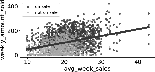
This is very strong evidence that your hypothesis $E\left[Y_0\right|T=1]>E\left[Y_0\right|T=0]$ was correct. There is an upward bias, as both the number of businesses with price cuts ($T=1$) and the outcome of those businesses, had they not done any sale ($Y_0$ for those businesses), would go up with business size.

If you’ve ever heard about Simpson’s Paradox, this bias is like a less extreme version of it. In Simpson’s Paradox, the relationship between two variables is initially positive, but, once you adjust for a third variable, it becomes negative. In our case, bias is not so extreme as to flip the sign of the association (see Figure 1-3). Here, you start with a situation where the association between price cuts and amount sold is too high and controlling for a third variable reduces the size of that association. If you zoom in inside businesses of the same size, the relationship between price cuts and amount sold decreases, but remains positive.

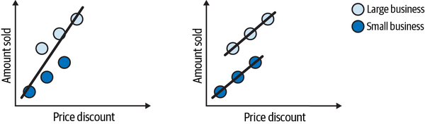
Figure 1-3. How bias relates to Simpson’s Paradox

Once again, this is so important that I think it is worth going over it again, now with some images. They are not realistic, but they do a good job of explaining the issue with bias. Let’s suppose you have a variable indicating the size of the business. If you plot the amount sold against size, you’ll see an increasing trend, where the bigger the size, the more the business sells. Next, you color the dots according to the treatment: white dots are businesses that cut their prices and black dots are businesses that didn’t do that. If you simply compare the average amount sold between treated and untreated business, this is what you’ll get:

Notice how the difference in amount sold between the two groups can (and probably does) have two causes:

1. The treatment effect. The increase in the amount sold, which is caused by the price cut.

2. The business size. Bigger businesses are able both to sell more and do more price cuts. This source of difference between the treated and untreated is not due to the price cut.

The challenge in causal inference is untangling both causes.

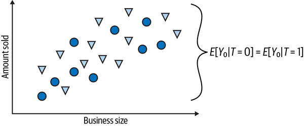
Contrast this with what you would see if you add both potential outcomes to the picture (counterfactual outcomes are denoted as triangles). The individual treatment effect is the difference between the unit’s outcome and another theoretical outcome that the same unit would have if it got the alternative treatment. The average treatment effect you would like to estimate is the average difference between the potential outcomes for each individual unit, $Y_1-Y_0$. These individual differences are much smaller than the difference you saw in the previous plot, between treated and untreated groups. The reason for this is bias, which is depicted in the right plot:

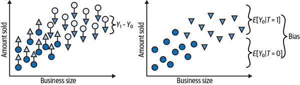
You can represent the bias by setting everyone to not receive the treatment. In this case, you are only left with the $Y_0$ potential outcome. Then, you can see how the treated and untreated groups differ on those potential outcomes under no treatment. If they do, something other than the treatment is causing the treated and untreated to be different. This is precisely the bias I’ve been talking about. It is what shadows the true treatment effect.

Identifying the Treatment Effect

Now that you understand the problem, it’s time to look at the (or at least one) solution. Identification is the first step in any causal inference analysis. You’ll see much more of it in Chapter 3, but for now, it’s worth knowing what it is. Remember that you can’t observe the causal quantities, since only one potential outcome is observable. You can’t directly estimate something like $E[Y_1-Y_0]$, since you can’t observe this difference for any data point. But perhaps you can find some other quantity, which is observable, and can be used to recover the causal quantity you care about. This is the process of identification: figuring out how to recover causal quantities from observable data. For instance, if, by some sort of miracle, $E\left[Y\right|T=t]$ managed to recover $E\left[Y_t\right]$ (identify $E\left[Y_t\right]$), you would be able to get $E[Y_1-Y_0]$ by simply estimating $E\left[Y\right|T=1]-E[Y|T=0]$. This can be done by estimating the average outcome for the treated and untreated, which are both observed quantities.

See Also

In the past decade (2010–2020), an entire body of knowledge on causal identification was popularized by Judea Pearl and his team, as an attempt to unify the causal inference language. I use some of that language in this chapter—although probably an heretical version of it—and I’ll cover more about it in Chapter 3. If you want to learn more about it, a short yet really cool paper to check out is “Causal Inference and Data Fusion in Econometrics,” by Paul Hünermund and Elias Bareinboim.

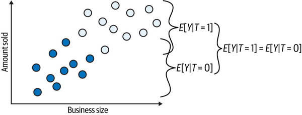
You can also see identification as the process of getting rid of bias. Using potential outcomes, you can also say what would be necessary to make association equal to causation. If $E\left[Y_0\right|T=0]=E\left[Y_0\right|T=1]$, then, association IS CAUSATION! Understanding this is not just remembering the equation. There is a strong intuitive argument here. To say that $E\left[Y_0\right|T=0]=E\left[Y_0\right|T=1]$ is to say that treatment and control group are comparable regardless of the treatment. Mathematically, the bias term would vanish, leaving only the effect on the treated:

$E\left[Y\right|T=1]-E\left[Y\right|T=0]=E[Y_1-Y_0|T=1]=ATT$

Also, if the treated and the untreated respond similarly to the treatment, that is, $E[Y_1-Y_0|T=1]=E[Y_1-Y_0|T=0]$, then (pay close attention), difference in means BECOMES the average causal effect:

$E\left[Y\right|T=1]-E\left[Y\right|T=0]=ATT=ATE=E[Y_1-Y_0]$

Despite the seemingly fancy-schmancy math here, all it’s saying is that once you make treated and control group interchangeable, expressing the causal effect in terms of observable quantities in the data becomes trivial. Applying this to our example, if businesses that do and don’t cut prices are similar to each other—that is, exchangeable—then, the difference in amount sold between the ones having sales and those not having sales can be entirely attributed to the price cut.

The Independence Assumption

This exchangeability is the key assumption in causal inference. Since it’s so important, different scientists found different ways to state it. I’ll start with one way, probably the most common, which is the independence assumption. Here, I’ll say that the potential outcomes are independent of the treatment: $(Y_0,Y_1)\perp T$.

This independence means that $E\left[Y_0\right|T]=E\left[Y_0\right]$, or, in other words, that the treatment gives you no information about the potential outcomes. The fact that a unit was treated doesn’t mean it would have a lower or higher outcome, had it not been treated ($Y_0$). This is just another way of saying that $E\left[Y_0\right|T=1]=E\left[Y_0\right|T=0]$. In our business example, it simply means that you wouldn’t be able to tell apart the businesses that chose to engage in sales from those that didn’t, had they all not done any sales. Except for the treatment and its effect on the outcome, they would be similar to each other. Similarly, $E\left[Y_1\right|T]=E\left[Y_1\right]$ means that you also wouldn’t be able to tell them apart, had they all engaged in sales. Simply put, it means that treated and untreated groups are comparable and indistinguishable, regardless of whether they all received the treatment or not.

Identification with Randomization

Here, you are treating independence as an assumption. That is, you know you need to make associations equal to causation, but you have yet to learn how to make this condition hold. Recall that a causal inference problem is often broken down into two steps:

1. Identification, where you figure out how to express the causal quantity of interest in terms of observable data.

2. Estimation, where you actually use data to estimate the causal quantity identified earlier.

To illustrate this process with a very simple example, let’s suppose that you can randomize the treatment. I know I said earlier that in the online marketplace you work for, businesses had full autonomy on setting prices, but you can still find a way to randomize the treatment $IsOnSales$. For instance, let’s say that you negotiate with the businesses the right to force them to cut prices, but the marketplace will pay for the price difference you’ve forced. OK, so suppose you now have a way to randomize sales, so what? This is a huge deal, actually!

First, randomization ties the treatment assignment to a coin flip, so variations in it become completely unrelated to any other factors in the causal mechanism:

$$\begin{array}{c}\hfill IsOnSales\leftarrow rand\left(t\right)\\ \hfill AmountSold\leftarrow f_y(IsOnSales,u_y)\end{array}$$

Under randomization $u_t$ vanished from our model since the assignment mechanism of the treatment became fully known. Moreover, since the treatment is random, it becomes independent from anything, including the potential outcomes. Randomization pretty much forces independence to hold.

To make this crystal clear, let’s see how randomization pretty much annihilates bias, starting before the treatment assignment. The first image shows the world of potential outcomes (triangles) yet to be realized. This is depicted by the image on the left:

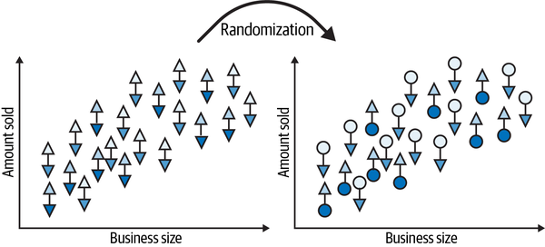
Then, at random, the treatment materializes one or the other potential outcome.

Randomized Versus Observational

In causal inference, we use the term randomized to talk about data where the treatment was randomized or when the assignment mechanism is fully known and nondeterministic. In contrast to that, the term observational is used to describe data where you can see who got what treatment, but you don’t know how that treatment was assigned.

Next, let’s get rid of the clutter, removing the unrealized potential outcomes (triangles). Now you can compare the treated to the untreated:

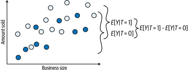
In this case, the difference in the outcome between treated and untreated is the average causal effect. This happens because there is no other source of difference between them other than the treatment itself. Therefore, all the differences you see must be attributed to the treatment. Or, simply put, there is no bias. If you set everyone to not receive the treatment so that you only observe the $Y_0$s, you would find no difference between the treated and untreated groups:

This is what the herculean task of causal identification is all about. It’s about finding clever ways of removing bias and making the treated and the untreated comparable so that all the difference you see can be attributed to the treatment effect. Importantly, identification is only possible if you know (or are willing to assume) something about the data-generating process. Usually, how the treatment was distributed or assigned. This is why I said earlier that data alone cannot answer causal questions. Sure, data is important for estimating the causal effect. But, besides data, you’ll always require a statement about how the data—specifically, the treatment—came to be. You get that statement using your expert knowledge or by intervening in the world, influencing the treatment and observing how the outcome changes in response.

An Incredible Membership Program

A big online retailer implemented a membership program, where members pay an extra fee to have access to more discounts, faster deliveries, return fee waiver, and amazing customer service. To understand the impact of the program, the company rolled it out to a random sample of the customers, which could opt in for paying the fee to get the membership benefits. After a while, they saw that customers in the membership program were much more profitable than those in the control group. Customers not only bought from the company, but they also spent less time with customer service. Should we then say that the membership program was a huge success in increasing sales and decreasing time spent serving customers?

Not really. Although the eligibility to the program was randomized, the random chunk that could opt in still self-selected into the program. In other words, randomization of program eligibility ensures that people who were able to get the program are comparable to those that weren’t. But, out of the eligible, only a fraction choose to participate. This choice was not random. Probably, only the more engaged customers chose to participate, while the casual ones dropped out. So, even though eligibility to the program was randomized, participation in the program was not. The result is that those that participated are not comparable to those that didn’t.

If you think about it, out of the eligible customers, the ones that actually chose to participate probably opted in for the program precisely because they already spent a lot in the online company, which made the extra discounts something worth paying for. This would imply that $E\left[Revenue{s}_0\right|OptIn=1]>E\left[Revenue{s}_0\right|OptIn=0]$, meaning those customers that opted in probably generated more revenues regardless of the program.

Ultimately, causal inference is about figuring out how the world works, stripped of all delusions and misinterpretations. And now that you understand this, you can move forward to mastering some of the most powerful methods to remove bias, the instruments of the brave and true, to identify the causal effect.

Key Ideas

You’ve learned the mathematical language that we’ll use to talk about causal inference in the rest of this book. Importantly, you’ve learned the definition of potential outcome as the outcome you would observe for a unit had that unit taken a specific treatment $T=t$:

$$Y_{ti}=Y_i|do(T_i=t)$$

Potential outcomes were very useful in understanding why association is different from causation. Namely, when treated and untreated are different due to reasons other than the treatment, $E\left[Y_0\right|T=1]\ne E\left[Y_0\right|T=0]$, and the comparison between both groups will not yield the true causal effect, but a biased estimate. We also used potential outcomes to see what we would need to make association equal to causation:

$$(Y_0,Y_1)\perp T$$

When treated and control groups are interchangeable or comparable, like when we randomize the treatment, a simple comparison between the outcome of the treated and untreated groups will yield the treatment effect:

$$E[Y_1-Y_0]=E\left[Y\right|T=1]-E\left[Y\right|T=0]$$

You also started to understand some of the key assumptions that you need to make when doing causal inference. For instance, in order to not have any bias when estimating the treatment effect, you assumed independence between the treatment assignment and the potential outcomes, $T\perp Y_t$.

You’ve also assumed that the treatment of one unit does not influence the outcome of another unit (SUTVA) and that all the versions of the treatment were accounted for (if $Y_i\left(t\right)=Y$, then $T_i=t$), when you defined the outcome $Y$ as a switch function between the potential outcomes:

$$Y_i=(1-T_i)Y_{0i}+T_i{Y}_{1i}$$

In general, it is always good to keep in mind that causal inference always requires assumptions. You need assumptions to go from the causal quantity you wish to know to the statistical estimator that can recover that quantity for you.