AI and Machine Learning for Coders

Chapter 1. Introduction to TensorFlow

When it comes to creating artificial intelligence (AI), machine learning (ML) and deep learning are a great place to begin. When getting started, however, it’s easy to get overwhelmed by the options and all the new terminology. This book aims to demystify things for programmers, taking you through writing code to implement concepts of machine learning and deep learning; and building models that behave more as a human does, with scenarios like computer vision, natural language processing (NLP), and more. Thus, they become a form of synthesized, or artificial, intelligence.

But when we refer to machine learning, what in fact is this phenomenon? Let’s take a quick look at that, and consider it from a programmer’s perspective before we go any further. After that, this chapter will show you how to install the tools of the trade, from TensorFlow itself to environments where you can code and debug your TensorFlow models.

What Is Machine Learning?

Before we get into the ins and outs of ML, let’s consider how it evolved from traditional programming. We’ll start by examining what traditional programming is, then consider cases where it is limited. Then we’ll see how ML evolved to handle those cases, and as a result has opened up new opportunities to implement new scenarios, unlocking many of the concepts of artificial intelligence.

Traditional programming involves us writing rules, expressed in a programming language, that act on data and give us answers. This applies just about everywhere that something can be programmed with code.

For example, consider a game like the popular Breakout. Code determines the movement of the ball, the score, and the various conditions for winning or losing the game. Think about the scenario where the ball bounces off a brick, like in Figure 1-1.

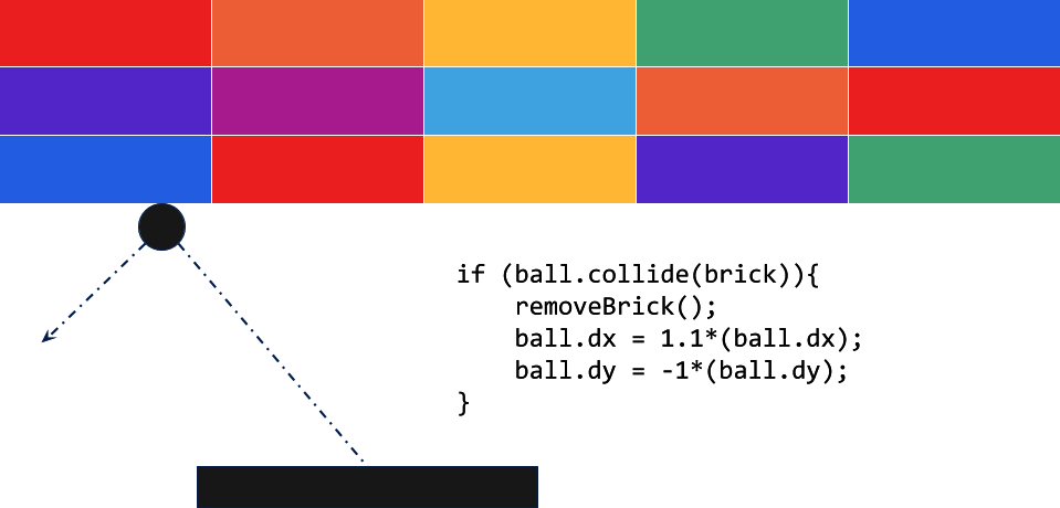
Figure 1-1. Code in a Breakout game

Here, the motion of the ball can be determined by its dx and dy properties. When it hits a brick, the brick is removed, and the velocity of the ball increases and changes direction. The code acts on data about the game situation.

Alternatively, consider a financial services scenario. You have data about a company’s stock, such as its current price and current earnings. You can calculate a valuable ratio called the P/E (for price divided by earnings) with code like that in Figure 1-2.

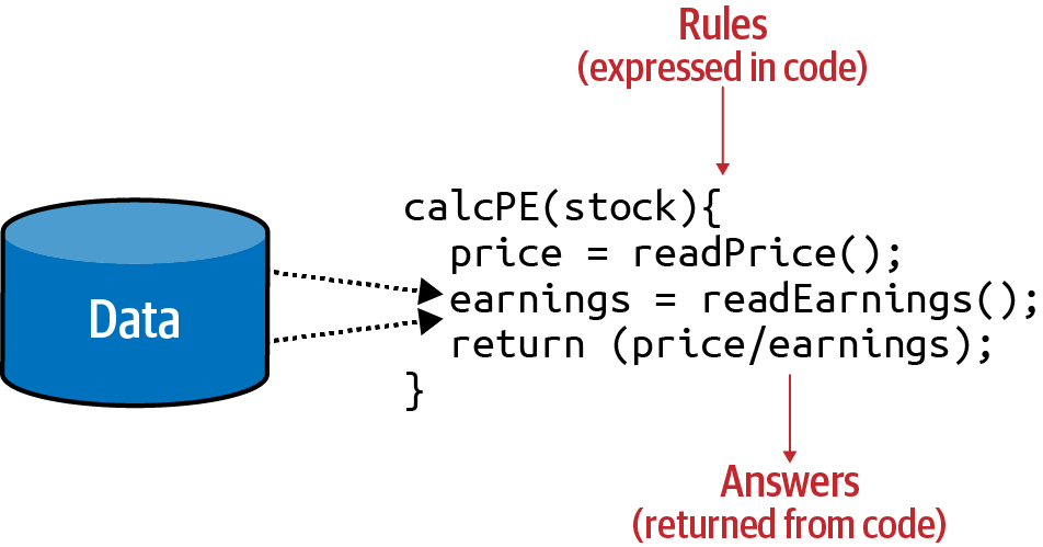
Figure 1-2. Code in a financial services scenario

Your code reads the price, reads the earnings, and returns a value that is the former divided by the latter.

If I were to try to sum up traditional programming like this into a single diagram, it might look like Figure 1-3.

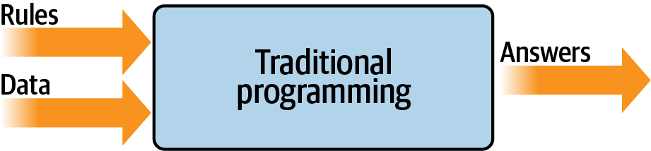
Figure 1-3. High-level view of traditional programming

As you can see, you have rules expressed in a programming language. These rules act on data, and the result is answers.

Limitations of Traditional Programming

The model from Figure 1-3 has been the backbone of development since its inception. But it has an inherent limitation: namely, that only scenarios that can be implemented are ones for which you can derive rules. What about other scenarios? Usually, they are infeasible to develop because the code is too complex. It’s just not possible to write code to handle them.

Consider, for example, activity detection. Fitness monitors that can detect our activity are a recent innovation, not just because of the availability of cheap and small hardware, but also because the algorithms to handle detection weren’t previously feasible. Let’s explore why.

Figure 1-4 shows a naive activity detection algorithm for walking. It can consider the person’s speed. If it’s less than a particular value, we can determine that they are probably walking.

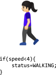
Figure 1-4. Algorithm for activity detection

Given that our data is speed, we could extend this to detect if they are running (Figure 1-5).

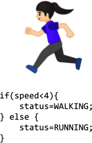
Figure 1-5. Extending the algorithm for running

As you can see, going by the speed, we might say if it is less than a particular value (say, 4 mph) the person is walking, and otherwise they are running. It still sort of works.

Now suppose we want to extend this to another popular fitness activity, biking. The algorithm could look like Figure 1-6.

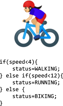
Figure 1-6. Extending the algorithm for biking

I know it’s naive in that it just detects speed—some people run faster than others, and you might run downhill faster than you cycle uphill, for example. But on the whole, it still works. However, what happens if we want to implement another scenario, such as golfing (Figure 1-7)?

Figure 1-7. How do we write a golfing algorithm?

We’re now stuck. How do we determine that someone is golfing using this methodology? The person might walk for a bit, stop, do some activity, walk for a bit more, stop, etc. But how can we tell this is golf?

Our ability to detect this activity using traditional rules has hit a wall. But maybe there’s a better way.

Enter machine learning.

From Programming to Learning

Let’s look back at the diagram that we used to demonstrate what traditional programming is (Figure 1-8). Here we have rules that act on data and give us answers. In our activity detection scenario, the data was the speed at which the person was moving; from that we could write rules to detect their activity, be it walking, biking, or running. We hit a wall when it came to golfing, because we couldn’t come up with rules to determine what that activity looks like.

Figure 1-8. The traditional programming flow

But what would happen if we were to flip the axes around on this diagram? Instead of us coming up with the rules, what if we were to come up with the answers, and along with the data have a way of figuring out what the rules might be?

Figure 1-9 shows what this would look like. We can consider this high-level diagram to define machine learning.

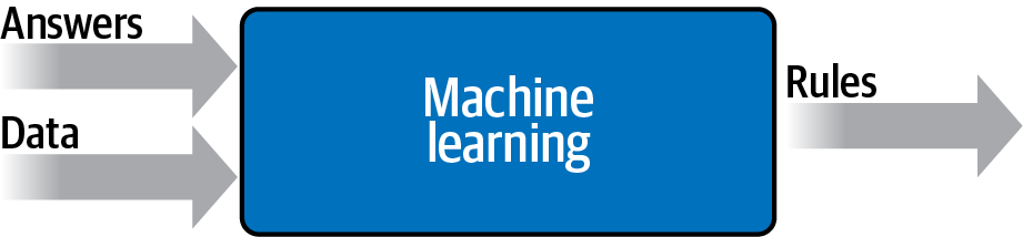
Figure 1-9. Changing the axes to get machine learning

So what are the implications of this? Well, now instead of us trying to figure out what the rules are, we get lots of data about our scenario, we label that data, and the computer can figure out what the rules are that make one piece of data match a particular label and another piece of data match a different label.

How would this work for our activity detection scenario? Well, we can look at all the sensors that give us data about this person. If they have a wearable that detects information such as heart rate, location, speed, etc.—and if we collect a lot of instances of this data while they’re doing different activities—we end up with a scenario of having data that says “This is what walking looks like,” “This is what running looks like,” and so on (Figure 1-10).

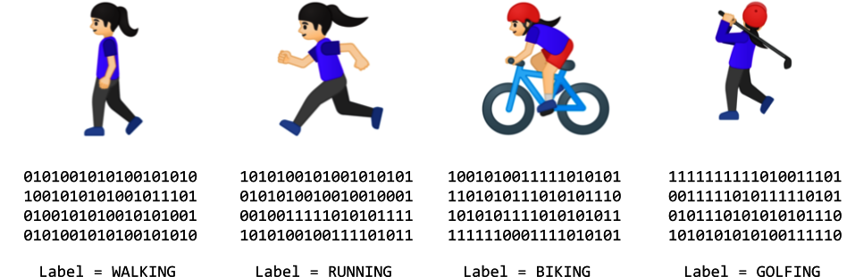
Figure 1-10. From coding to ML: gathering and labeling data

Now our job as programmers changes from figuring out the rules, to determining the activities, to writing the code that matches the data to the labels. If we can do this, then we can expand the scenarios that we can implement with code. Machine learning is a technique that enables us to do this, but in order to get started, we’ll need a framework—and that’s where TensorFlow enters the picture. In the next section we’ll take a look at what it is and how to install it, and then later in this chapter you’ll write your first code that learns the pattern between two values, like in the preceding scenario. It’s a simple “Hello World” scenario, but it has the same foundational code pattern that’s used in extremely complex ones.

The field of artificial intelligence is large and abstract, encompassing everything to do with making computers think and act the way human beings do. One of the ways a human takes on new behaviors is through learning by example. The discipline of machine learning can thus be thought of as an on-ramp to the development of artificial intelligence. Through it, a machine can learn to see like a human (a field called computer vision), read text like a human (natural language processing), and much more. We’ll be covering the basics of machine learning in this book, using the TensorFlow framework.

What Is TensorFlow?

TensorFlow is an open source platform for creating and using machine learning models. It implements many of the common algorithms and patterns needed for machine learning, saving you from needing to learn all the underlying math and logic and enabling you to just to focus on your scenario. It’s aimed at everyone from hobbyists, to professional developers, to researchers pushing the boundaries of artificial intelligence. Importantly, it also supports deployment of models to the web, cloud, mobile, and embedded systems. We’ll be covering each of these scenarios in this book.

The high-level architecture of TensorFlow can be seen in Figure 1-11.

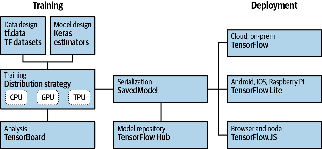
Figure 1-11. TensorFlow high-level architecture

The process of creating machine learning models is called training. This is where a computer uses a set of algorithms to learn about inputs and what distinguishes them from each other. So, for example, if you want a computer to recognize cats and dogs, you can use lots of pictures of both to create a model, and the computer will use that model to try to figure out what makes a cat a cat, and what makes a dog a dog. Once the model is trained, the process of having it recognize or categorize future inputs is called inference.

So, for training models, there are several things that you need to support. First is a set of APIs for designing the models themselves. With TensorFlow there are three main ways to do this: you can code everything by hand, where you figure out the logic for how a computer can learn and then implement that in code (not recommended); you can use built-in estimators, which are already-implemented neural networks that you can customize; or you can use Keras, a high-level API that allows you to encapsulate common machine learning paradigms in code. This book will primarily focus on using the Keras APIs when creating models.

There are many ways to train a model. For the most part, you’ll probably just use a single chip, be it a central processing unit (CPU) , a graphics processing unit (GPU), or something new called a tensor processing unit (TPU). In more advanced working and research environments, parallel training across multiple chips can be used, employing a distribution strategy where training spans multiple chips. TensorFlow supports this too.

The lifeblood of any model is its data. As discussed earlier, if you want to create a model that can recognize cats and dogs, it needs to be trained with lots of examples of cats and dogs. But how can you manage these examples? You’ll see, over time, that this can often involve a lot more coding than the creation of the models themselves. TensorFlow ships with APIs to try to ease this process, called TensorFlow Data Services. For learning, they include lots of preprocessed datasets that you can use with a single line of code. They also give you the tools for processing raw data to make it easier to use.

Beyond creating models, you’ll also need to be able to get them into people’s hands where they can be used. To this end, TensorFlow includes APIs for serving, where you can provide model inference over an HTTP connection for cloud or web users. For models to run on mobile or embedded systems, there’s TensorFlow Lite, which provides tools for model inference on Android and iOS as well as Linux-based embedded systems such as a Raspberry Pi. A fork of TensorFlow Lite, called TensorFlow Lite Micro (TFLM), also provides inference on microcontrollers through an emerging concept known as TinyML. Finally, if you want to provide models to your browser or Node.js users, TensorFlow.js offers the ability to train and execute models in this way.

Next, I’ll show you how to install TensorFlow so that you can get started creating and using ML models with it.

Using TensorFlow

In this section, we’ll look at the three main ways that you can install and use TensorFlow. We’ll start with how to install it on your developer box using the command line. We’ll then explore using the popular PyCharm IDE (integrated development environment) to install TensorFlow. Finally, we’ll look at Google Colab and how it can be used to access TensorFlow code with a cloud-based backend in your browser.

Installing TensorFlow in Python

TensorFlow supports the creation of models using multiple languages, including Python, Swift, Java, and more. In this book we’ll focus on using Python, which is the de facto language for machine learning due to its extensive support for mathematical models. If you don’t have it already, I strongly recommend you visit Python to get up and running with it, and learnpython.org to learn the Python language syntax.

With Python there are many ways to install frameworks, but the default one supported by the TensorFlow team is pip.

So, in your Python environment, installing TensorFlow is as easy as using:

pip install tensorflow

Note that starting with version 2.1, this will install the GPU version of TensorFlow by default. Prior to that, it used the CPU version. So, before installing, make sure you have a supported GPU and all the requisite drivers for it. Details on this are available at TensorFlow.

If you don’t have the required GPU or drivers, you can still install the CPU version of TensorFlow on any Linux, PC, or Mac with:

pip install tensorflow-cpu

Once you’re up and running, you can test your TensorFlow version with the following code:

import tensorflow as tf
print(tf.__version__)

You should see output like that in Figure 1-12. This will print the currently running version of TensorFlow—here you can see that version 2.0.0 is installed.

Figure 1-12. Running TensorFlow in Python

Using TensorFlow in PyCharm

I’m particularly fond of using the free community version of PyCharm for building models using TensorFlow. PyCharm is useful for many reasons, but one of my favorites is that it makes the management of virtual environments easy. This means you can have Python environments with versions of tools such as TensorFlow that are specific to your particular project. So, for example, if you want to use TensorFlow 2.0 in one project and TensorFlow 2.1 in another, you can separate these with virtual environments and not have to deal with installing/uninstalling dependencies when you switch. Additionally, with PyCharm you can do step-by-step debugging of your Python code—a must, especially if you’re just getting started.

For example, in Figure 1-13 I have a new project that is called example1, and I’m specifying that I am going to create a new environment using Conda. When I create the project I’ll have a clean new virtual Python environment into which I can install any version of TensorFlow I want.

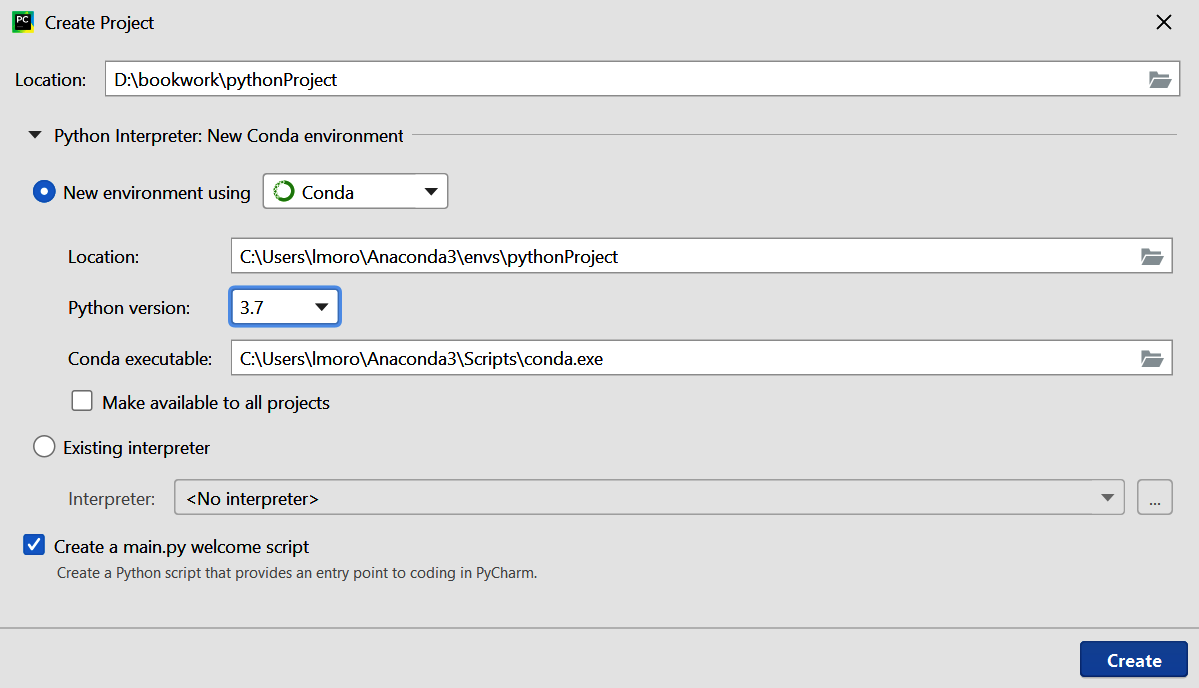
Figure 1-13. Creating a new virtual environment using PyCharm

Once you’ve created a project, you can open the File → Settings dialog and choose the entry for “Project: <your project name>” from the menu on the left. You’ll then see choices to change the settings for the Project Interpreter and the Project Structure. Choose the Project Interpreter link, and you’ll see the interpreter that you’re using, as well as a list of packages that are installed in this virtual environment (Figure 1-14).

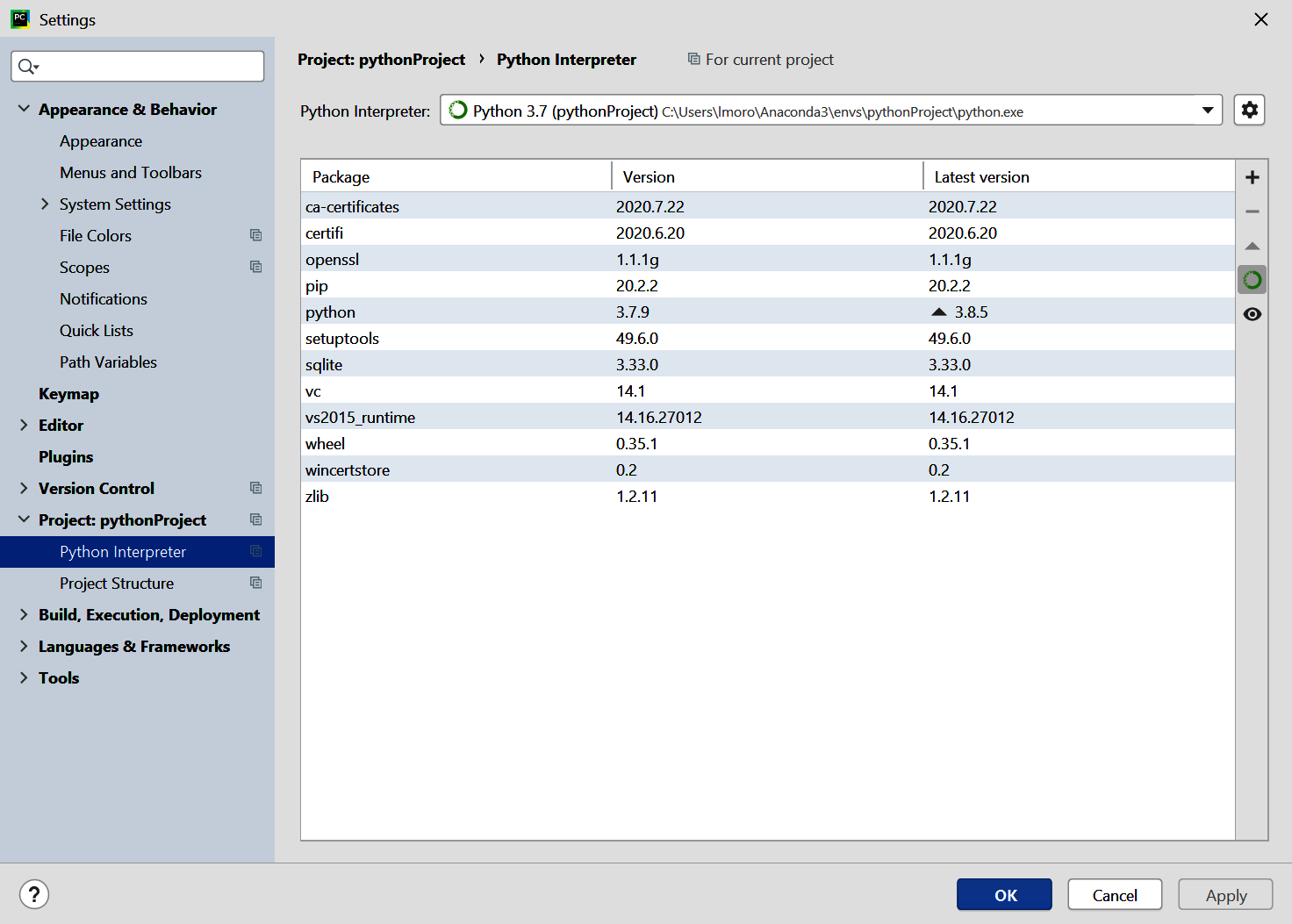
Figure 1-14. Adding packages to a virtual environment

Click the + button on the right, and a dialog will open showing the packages that are currently available. Type “tensorflow” into the search box and you’ll see all available packages with “tensorflow” in the name (Figure 1-15).

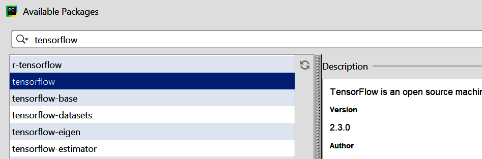
Figure 1-15. Installing TensorFlow with PyCharm

Once you’ve selected TensorFlow, or any other package you want to install, and then click the Install Package button, PyCharm will do the rest.

Once TensorFlow is installed, you can now write and debug your TensorFlow code in Python.

Using TensorFlow in Google Colab

Another option, which is perhaps easiest for getting started, is to use Google Colab, a hosted Python environment that you can access via a browser. What’s really neat about Colab is that it provides GPU and TPU backends so you can train models using state-of-the-art hardware at no cost.

When you visit the Colab website, you’ll be given the option to open previous Colabs or start a new notebook, as shown in Figure 1-16.

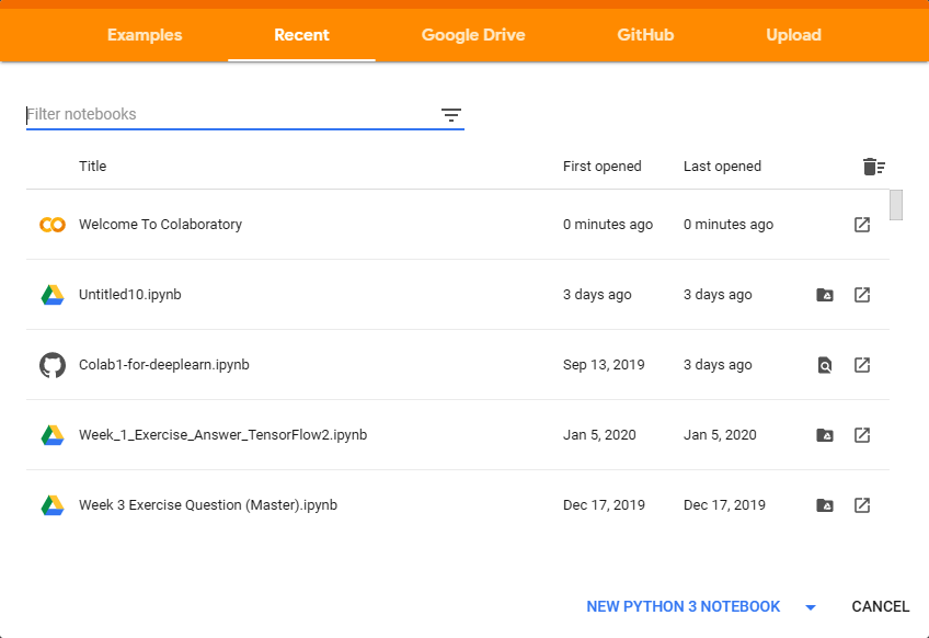
Figure 1-16. Getting started with Google Colab

Clicking the New Python 3 Notebook link will open the editor, where you can add panes of code or text (Figure 1-17). You can execute the code by clicking the Play button (the arrow) to the left of the pane.

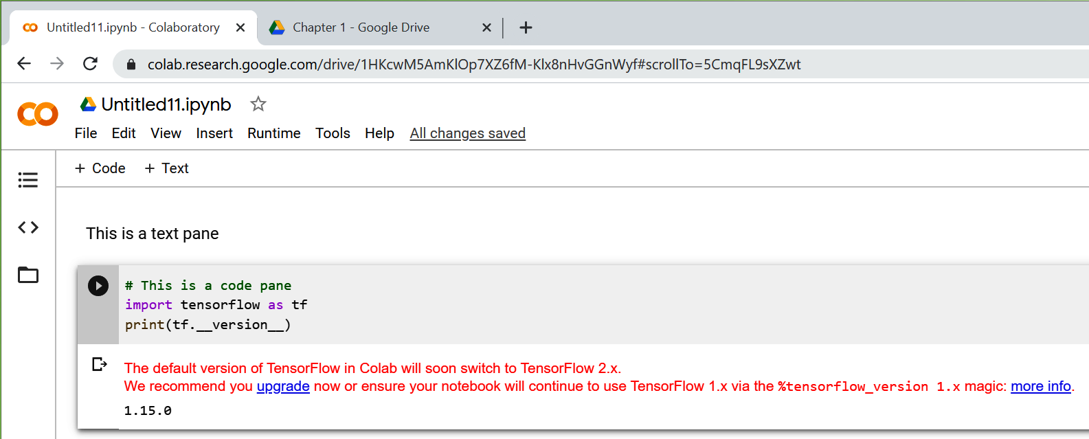
Figure 1-17. Running TensorFlow code in Colab

It’s always a good idea to check the TensorFlow version, as shown here, to be sure you’re running the correct version. Often Colab’s built-in TensorFlow will be a version or two behind the latest release. If that’s the case you can update it with pip install as shown earlier, by simply using a block of code like this:

!pip install tensorflow==2.1.0

Once you run this command, your current environment within Colab will use the desired version of TensorFlow.

Getting Started with Machine Learning

As we saw earlier in the chapter, the machine learning paradigm is one where you have data, that data is labeled, and you want to figure out the rules that match the data to the labels. The simplest possible scenario to show this in code is as follows. Consider these two sets of numbers:

X = –1, 0, 1, 2, 3, 4
Y = –3, –1, 1, 3, 5, 7

There’s a relationship between the X and Y values (for example, if X is –1 then Y is –3, if X is 3 then Y is 5, and so on). Can you see it?

After a few seconds you probably saw that the pattern here is Y = 2X – 1. How did you get that? Different people work it out in different ways, but I typically hear the observation that X increases by 1 in its sequence, and Y increases by 2; thus, Y = 2X +/– something. They then look at when X = 0 and see that Y = –1, so they figure that the answer could be Y = 2X – 1. Next they look at the other values and see that this hypothesis “fits,” and the answer is Y = 2X – 1.

That’s very similar to the machine learning process. Let’s take a look at some TensorFlow code that you could write to have a neural network do this figuring out for you.

Here’s the full code, using the TensorFlow Keras APIs. Don’t worry if it doesn’t make sense yet; we’ll go through it line by line:

import tensorflow as tf
import numpy as np
from tensorflow.keras import Sequential
from tensorflow.keras.layers import Dense

model = Sequential([Dense(units=1, input_shape=[1])])
model.compile(optimizer='sgd', loss='mean_squared_error')

xs = np.array([-1.0, 0.0, 1.0, 2.0, 3.0, 4.0], dtype=float)
ys = np.array([-3.0, -1.0, 1.0, 3.0, 5.0, 7.0], dtype=float)

model.fit(xs, ys, epochs=500)

print(model.predict([10.0]))

Let’s start with the first line. You’ve probably heard of neural networks, and you’ve probably seen diagrams that explain them using layers of interconnected neurons, a little like Figure 1-18.

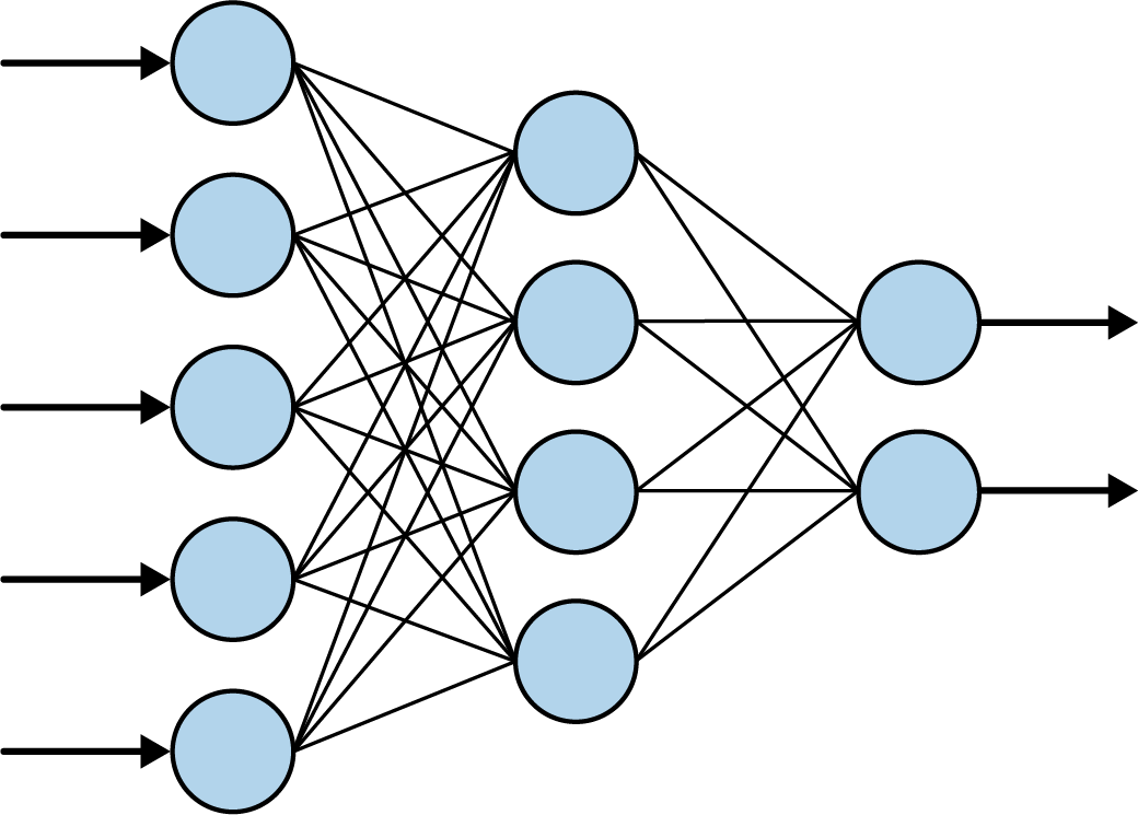
Figure 1-18. A typical neural network

When you see a neural network like this, consider each of the “circles” to be a neuron, and each of the columns of circles to be a layer. So, in Figure 1-18, there are three layers: the first has five neurons, the second has four, and the third has two.

If we look back at our code and look at just the first line, we’ll see that we’re defining the simplest possible neural network. There’s only one layer, and it contains only one neuron:

model = Sequential([Dense(units=1, input_shape=[1])])

When using TensorFlow, you define your layers using Sequential. Inside the Sequential, you then specify what each layer looks like. We only have one line inside our Sequential, so we have only one layer.

You then define what the layer looks like using the keras.layers API. There are lots of different layer types, but here we’re using a Dense layer. “Dense” means a set of fully (or densely) connected neurons, which is what you can see in Figure 1-18 where every neuron is connected to every neuron in the next layer. It’s the most common form of layer type. Our Dense layer has units=1 specified, so we have just one dense layer with one neuron in our entire neural network. Finally, when you specify the first layer in a neural network (in this case, it’s our only layer), you have to tell it what the shape of the input data is. In this case our input data is our X, which is just a single value, so we specify that that’s its shape.

The next line is where the fun really begins. Let’s look at it again:

model.compile(optimizer='sgd', loss='mean_squared_error')

If you’ve done anything with machine learning before, you’ve probably seen that it involves a lot of mathematics. If you haven’t done calculus in years it might have seemed like a barrier to entry. Here’s the part where the math comes in—it’s the core to machine learning.

In a scenario such as this one, the computer has no idea what the relationship between X and Y is. So it will make a guess. Say for example it guesses that Y = 10X + 10. It then needs to measure how good or how bad that guess is. That’s the job of the loss function.

It already knows the answers when X is –1, 0, 1, 2, 3, and 4, so the loss function can compare these to the answers for the guessed relationship. If it guessed Y = 10X + 10, then when X is –1, Y will be 0. The correct answer there was –3, so it’s a bit off. But when X is 4, the guessed answer is 50, whereas the correct one is 7. That’s really far off.

Armed with this knowledge, the computer can then make another guess. That’s the job of the optimizer. This is where the heavy calculus is used, but with TensorFlow, that can be hidden from you. You just pick the appropriate optimizer to use for different scenarios. In this case we picked one called sgd, which stands for stochastic gradient descent—a complex mathematical function that, when given the values, the previous guess, and the results of calculating the errors (or loss) on that guess, can then generate another one. Over time, its job is to minimize the loss, and by so doing bring the guessed formula closer and closer to the correct answer.

Next, we simply format our numbers into the data format that the layers expect. In Python, there’s a library called Numpy that TensorFlow can use, and here we put our numbers into a Numpy array to make it easy to process them:

xs = np.array([-1.0, 0.0, 1.0, 2.0, 3.0, 4.0], dtype=float)
ys = np.array([-3.0, -1.0, 1.0, 3.0, 5.0, 7.0], dtype=float)

The learning process will then begin with the model.fit command, like this:

model.fit(xs, ys, epochs=500)

You can read this as “fit the Xs to the Ys, and try it 500 times.” So, on the first try, the computer will guess the relationship (i.e., something like Y = 10X + 10), and measure how good or bad that guess was. It will then feed those results to the optimizer, which will generate another guess. This process will then be repeated, with the logic being that the loss (or error) will go down over time, and as a result the “guess” will get better and better.

Figure 1-19 shows a screenshot of this running in a Colab notebook. Take a look at the loss values over time.

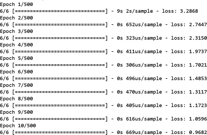
Figure 1-19. Training the neural network

We can see that over the first 10 epochs, the loss went from 3.2868 to 0.9682. That is, after only 10 tries, the network was performing three times better than with its initial guess. Then take a look at what happens by the five hundredth epoch (Figure 1-20).

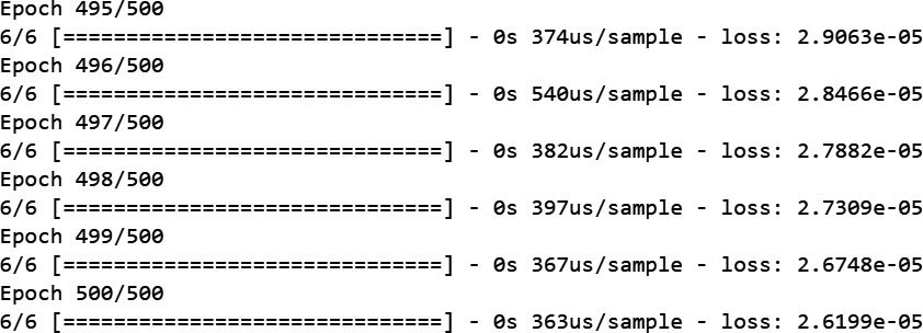
Figure 1-20. Training the neural network—the last five epochs

We can now see the loss is 2.61 × 10^-5. The loss has gotten so small that the model has pretty much figured out that the relationship between the numbers is Y = 2X – 1. The machine has learned the pattern between them.

Our last line of code then used the trained model to get a prediction like this:

print(model.predict([10.0]))

Note

The term prediction is typically used when dealing with ML models. Don’t think of it as looking into the future, though! This term is used because we’re dealing with a certain amount of uncertainty. Think back to the activity detection scenario we spoke about earlier. When the person was moving at a certain speed, she was probably walking. Similarly, when a model learns about the patterns between two things it will tell us what the answer probably is. In other words, it is predicting the answer. (Later you’ll also learn about inference, where the model is picking one answer among many, and inferring that it has picked the correct one.)

What do you think the answer will be when we ask the model to predict Y when X is 10? You might instantly think 19, but that’s not correct. It will pick a value very close to 19. There are several reasons for this. First of all, our loss wasn’t 0. It was still a very small amount, so we should expect any predicted answer to be off by a very small amount. Secondly, the neural network is trained on only a small amount of data—in this case only six pairs of (X,Y) values.

The model only has a single neuron in it, and that neuron learns a weight and a bias, so that Y = WX + B. This looks exactly like the relationship Y = 2X – 1 that we want, where we would want it to learn that W = 2 and B = –1. Given that the model was trained on only six items of data, the answer could never be expected to be exactly these values, but something very close to them.

Run the code for yourself to see what you get. I got 18.977888 when I ran it, but your answer may differ slightly because when the neural network is first initialized there’s a random element: your initial guess will be slightly different from mine, and from a third person’s.

Seeing What the Network Learned

This is obviously a very simple scenario, where we are matching Xs to Ys in a linear relationship. As mentioned in the previous section, neurons have weight and bias parameters that they learn, which makes a single neuron fine for learning a relationship like this: namely, when Y = 2X – 1, the weight is 2 and the bias is –1. With TensorFlow we can actually take a look at the weights and biases that are learned, with a simple change to our code like this:

import tensorflow as tf
import numpy as np
from tensorflow.keras import Sequential
from tensorflow.keras.layers import Dense

l0 = Dense(units=1, input_shape=[1])
model = Sequential([l0])
model.compile(optimizer='sgd', loss='mean_squared_error')

xs = np.array([-1.0, 0.0, 1.0, 2.0, 3.0, 4.0], dtype=float)
ys = np.array([-3.0, -1.0, 1.0, 3.0, 5.0, 7.0], dtype=float)

model.fit(xs, ys, epochs=500)

print(model.predict([10.0]))
print("Here is what I learned: {}".format(l0.get_weights()))

The difference is that I created a variable called l0 to hold the Dense layer. Then, after the network finishes learning, I can print out the values (or weights) that the layer learned.

In my case, the output was as follows:

Here is what I learned: [array([[1.9967953]], dtype=float32), 
array([-0.9900647], dtype=float32)]

Thus, the learned relationship between X and Y was Y = 1.9967953X – 0.9900647.

This is pretty close to what we’d expect (Y = 2X – 1), and we could argue that it’s even closer to reality, because we are assuming that the relationship will hold for other values.

Summary

That’s it for your first “Hello World” of machine learning. You might be thinking that this seems like massive overkill for something as simple as determining a linear relationship between two values. And you’d be right. But the cool thing about this is that the pattern of code we’ve created here is the same pattern that’s used for far more complex scenarios. You’ll see these starting in Chapter 2, where we’ll explore some basic computer vision techniques—the machine will learn to “see” patterns in pictures, and identify what’s in them.