Query the planet: Geospatial big data analytics at Uber
A deep dive into Uber's engineering effort to optimize geospatial queries in Presto.
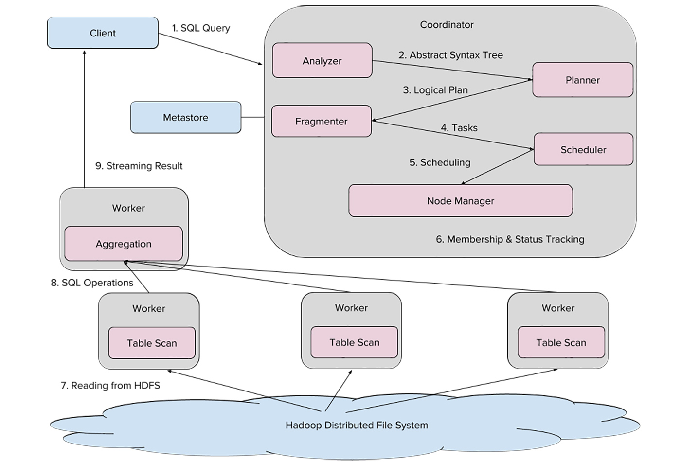 Uber’s Presto architecture (source: Courtesy of Zhenxiao Luo)
From determining the most convenient rider pickup points to predicting the fastest routes, Uber aims to use data-driven analytics to create seamless trip experiences. Within engineering, analytics inform decision-making processes across the board.
One of the distinct challenges for Uber is analyzing geospatial big data. City locations, trips, and event information, for instance, provide insights that can improve business decisions and better serve users. Geospatial data analysis is particularly challenging, especially in a big data scenario, such as computing how many rides start at a transit location, how many drivers are crossing state lines, and so on. For these analytical requests, we must achieve efficiency, usability, and scalability in order to meet user needs and business requirements.
To accomplish this, we use Presto in our production environment to process the big data powering our interactive SQL engine. In this article, we discuss our engineering effort to optimize geospatial queries in Presto.
Using Presto at Uber
We chose Presto as our system’s SQL engine because of its scalability, high performance, and smooth integration with Hadoop. These properties make it a good fit for many of our teams.
Presto architecture
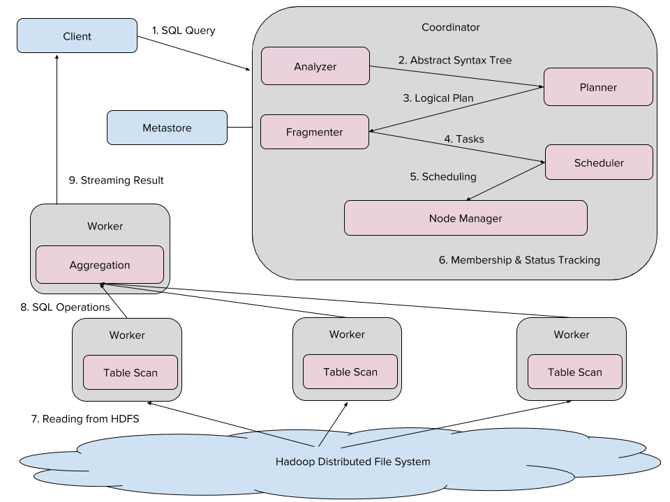
Uber’s Presto ecosystem is made up of a variety of nodes that process data stored in Hadoop. Each Presto cluster has one “coordinator” node that compiles SQL and schedules tasks, as well as a number of “worker” nodes that jointly execute tasks. As detailed in Figure 1, the client sends SQL queries to our Presto coordinator, whose analyzer compiles SQL into an Abstract Syntax Tree (AST).
From there, the planner compiles the AST into a query plan, optimizing it for a fragmenter that then segments the plan into tasks. Next, the scheduler assigns each task—either reading files from the Hadoop Distributed File System (HDFS) or conducting aggregations—to a specific worker, and the node manager tracks their progress. Finally, results of these tasks are streamed to the client.
Hadoop infrastructure and analytics
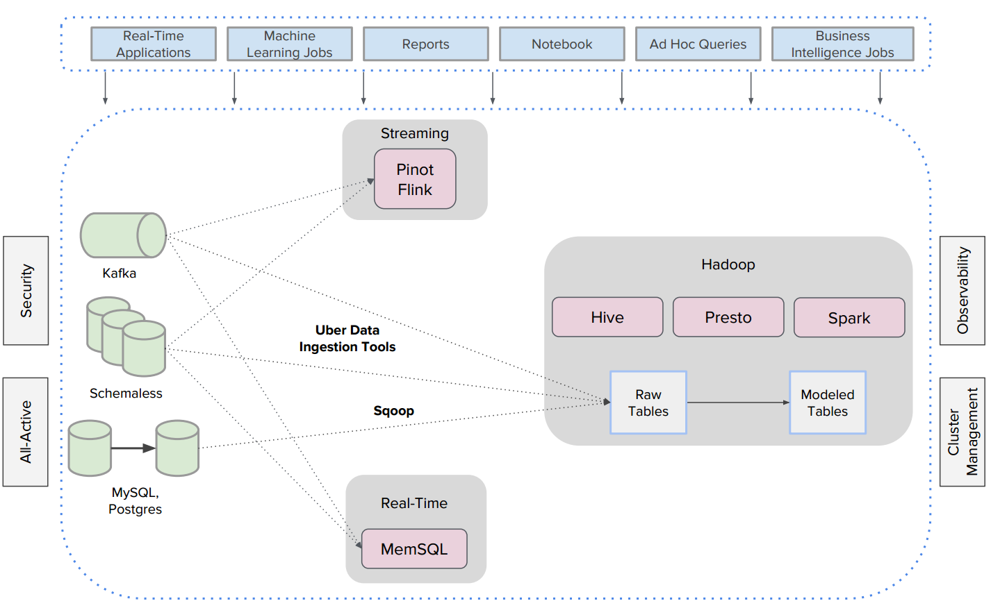
Analytic data sets at Uber are captured in our Hadoop warehouse, including event logs replicated by Kafka, service-oriented architecture tables built with MySQL and Postgres, and trip data stored in Schemaless. We run Flink, Pinot, and MemSQL for streaming and real-time analysis of this data.
The Hadoop Distributed File System (HDFS) is our data lake. In this ecosystem, event logs and trip data are ingested using Uber internal data ingestion tools, and service-oriented tables are copied to HDFS via Sqoop. With Uber Hoodie, Uber’s incremental updates and inserts library, data is first dumped into our HDFS as nested raw files, and then some of these raw tables are converted into modeled tables via extract, transform, load (ETL) jobs. While batch and ETL jobs run on Hive and Spark, near real-time interactive queries run on Presto.
This robust Hadoop infrastructure is integrated across Uber’s data centers, incorporating existing all-active, observability, cluster management, and security features.
Geospatial data model
Modeling geospatial data has distinct complexities. To model real-world cities and trips into simplified shapes and points represented in big data tables, we use the Well-Known Text (WKT) used in ESRI Geometry API to represent geometries.
Point
A point represents a single location in a two-dimensional space. Internally, we store each point as a pair of (longitude, latitude), e.g.:
POINT (77.3548351 28.6973627)
Polygon
We simply store a polygon as a collection of points, such that the start point and the end point match, e.g.:
POLYGON ((36.814155579 -1.3174386070000002, 36.814863682 -1.317545867, 36.814863682 -1.318221605, 36.813973188 -1.317910551, 36.814155579 -1.3174386070000002))
Geospatial Use Cases at Uber
At Uber, geospatial data is organized as geofences, where a geofence is either a polygon or a multi-polygon. We provide internal tools to create, edit, and delete geofences. Every few minutes, any geofence changes will be dumped into a Hadoop table, which is queryable by Presto. In this system, we have a trips table, which records trip start points and endpoints, as well as the cities table, which contains the city identification column city_id and its corresponding geofence column geo_shape.
Geospatial data is used for promotions, driver supply identification, and events regulation, among other use cases. For example, Uber could launch a promotion for free basketball tickets for riders who are taking Uber trips to a Warriors game. In this scenario, our engineer would create a new geofence that contains Oracle Arena Stadium, then write a Presto query to target all users who are taking trips to the stadium before the game for the promotion, and, then, randomly select the winner, as portrayed in Figure 3.

Challenges
To discern how many trips occur within a given city on a specific date, we run the following SQL query:
SELECT c.city_id, count(*)
FROM trips_table as t
JOIN city_table as c
ON st_contains(c.geo_shape, st_point(t.dest_lng, t.dest_lat))
WHERE datestr = ‘2017-08-01’
GROUP BY 1
st_point is the standard geo function to construct a two-dimensional point using longitude and latitude. st_contains is the standard geo function to compute whether a point is within a geo shape.
This query needs to compute st_contains for each point and geofence pair. For a real city, it is not uncommon to see its geofence composed of hundreds or thousands of points. The time cost of executing st_contains for one pair of point and geofence is proportional to the number of points in the geofence.
Given that millions of Uber trips are requested each day across hundreds of cities, this simple query could cost hundreds of millions of st_contains, which in turn computes hundreds of thousands Point-Point operations.
One simple query with a brute force Hive MapReduce execution could take days to complete!
Geospatial optimizations
This huge time commitment is insufficient for Uber’s use case. To ensure we provide optimal trip experiences for our users, we need to optimize how we processed this data.
QuadTree
Quadtrees represent a partition of space in two dimensions by decomposing the region into four quadrants, sub-quadrants, and so on until the contents of the cells meet some criterion of data occupancy. For example, in Figure 4, we built QuadTree to index a 4X4 square space.
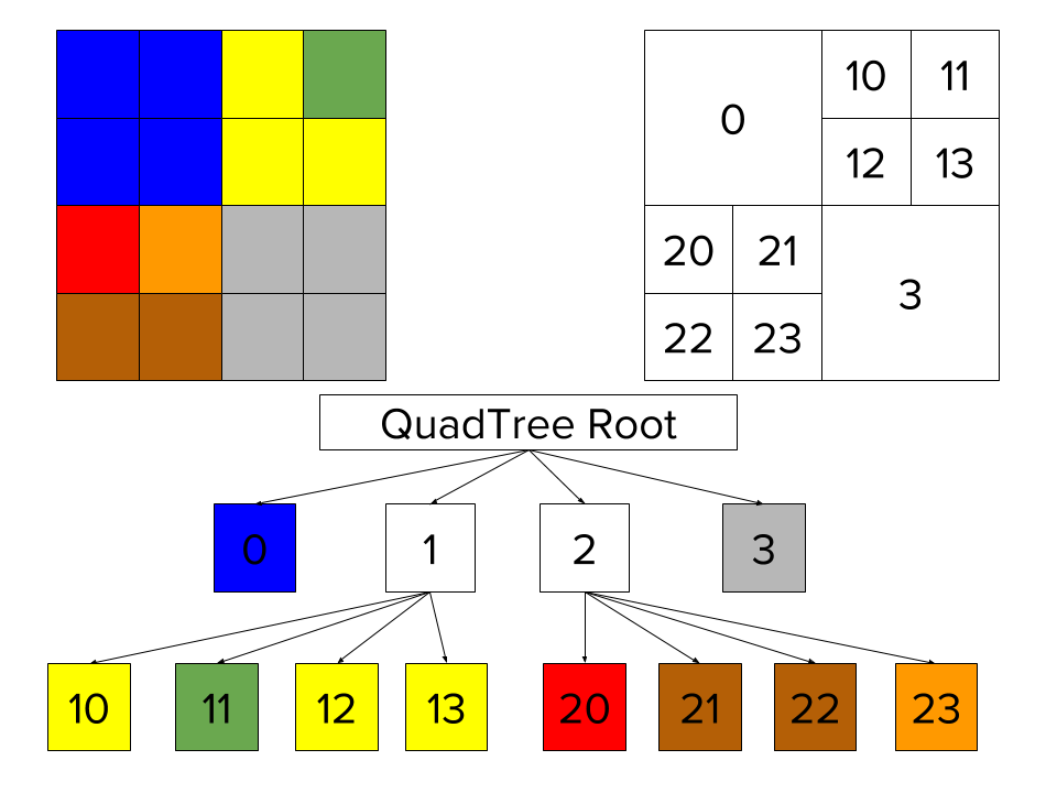
For our use case, we can use rectangles and squares to divide and index real city boundaries.
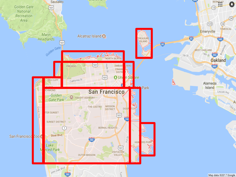
Using QuadTree, the majority of bounded rectangles that do not contain target point could be filtered out. We run geospatial functions (e.g., st_contains) only for rectangles that contain target point.
Presto Geospatial plugin
Using the Presto plugin framework, we implemented a Presto Geospatial plugin, which possesses a variety of geo-functions. One of them is a Presto Aggregation Function, build_geo_index, which serializes/deserializes geospatial polygons into a QuadTree.
During query execution, we build a QuadTree on the fly. QuadTree is used to filter out geofences that do not contain target point. During this phase, majority of geofences would be filtered out. Finally, we run st_contains for remaining geofences.
Presto query optimization
To improve usability, we added Presto query optimizations to automatically rewrite user queries into optimized ones, as portrayed in Figure 6.
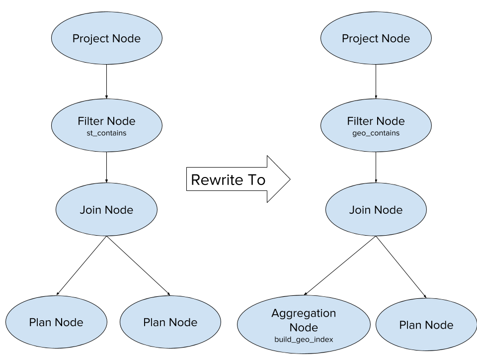
| Query Rewrite From | Query Rewrite To |
| SELECT c.city_id, count(*)
FROM trips_table as t JOIN city_table as c ON st_contains(c.geo_shape, st_point(t.dest_lng, t.dest_lat)) WHERE datestr = ‘2017-08-01’ GROUP BY 1 |
SELECT
geo_contains(st_point(t.dest_lng, t.dest_lat), geo_index) as city_id, count(*) FROM trips_table as t CROSS JOIN ( SELECT build_geo_index(city_id, geo_shape) as geo_index FROM city_table) WHERE datestr = ‘2017-08-01’ and city_id is not null GROUP BY 1 |
Production status
Presto GeoSpatial plugin is running in production at Uber. Among our GeoSpatial traffic, more than 90% is completed within five minutes. Compared with the brute force Hive MapReduce execution, our Presto Geospatial Plugin is more than 50X faster, leading to greater efficiency.
For more on our work in this space, check out our Uber Engineering Blog article on engineering data analytics using Presto and Parquet, and attend our talk at the Strata Data Conference in New York, September 25-28, 2017.
