Transfer learning from multiple pre-trained computer vision models
Using the keras TensorFlow abstraction library, the method is simple, easy to implement, and often produces surprisingly good results.
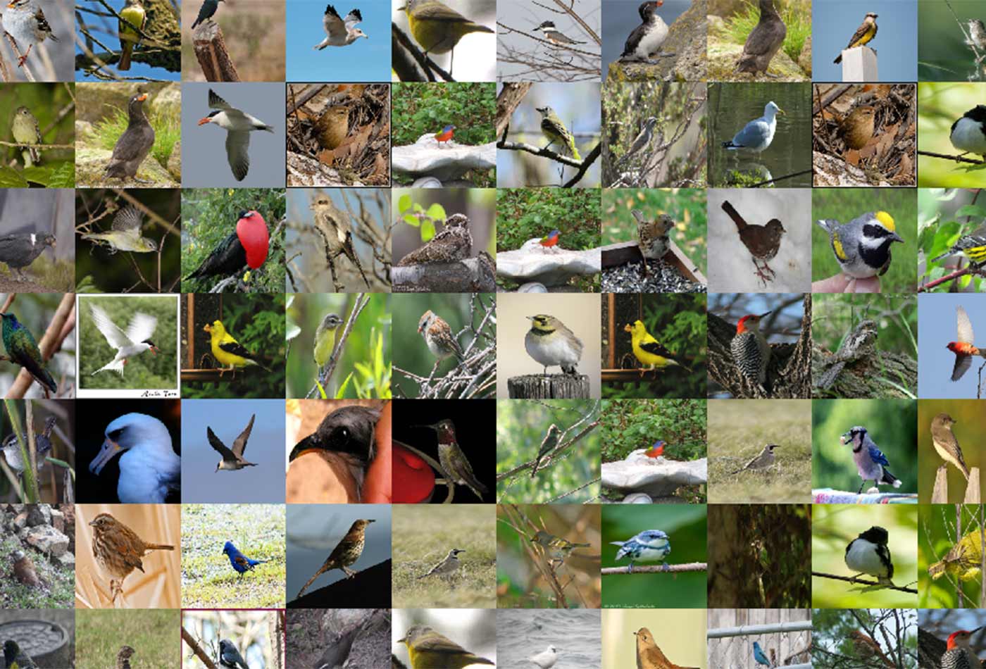
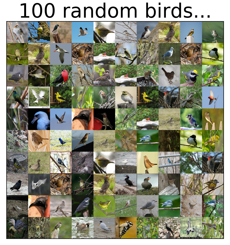
 Birds from the CUB-200 data set (source: Yehezkel Resheff, used with permission)
The multitude of methods jointly referred to as “deep learning” have disrupted the fields of machine learning and data science, rendering decades of engineering know-how almost completely irrelevant—or so common opinion would have it. Of all these, one method that stands out in its overwhelming simplicity, robustness, and usefulness is the transfer of learned representations. Especially for computer vision, this approach has brought about unparalleled ability, accessible to practitioners of all levels, and making previously insurmountable tasks as easy as from keras.applications import *.
Put simply, the method dictates that a large data set should be used in order to learn to represent the object of interest (image, time-series, customer, even a network) as a feature vector, in a way that lends itself to downstream data science tasks such as classification or clustering. Once learned, the representation machinery may then be used by other researchers, and for other data sets, almost regardless of the size of the new data or computational resources available.
In this blog post, we demonstrate the use of transfer learning with pre-trained computer vision models, using the keras TensorFlow abstraction library. The models we will use have all been trained on the large ImageNet data set, and learned to produce a compact representation of an image in the form of a feature vector. We will use this mechanism to learn a classifier for species of birds.
There are many ways to use pre-trained models, the choice of which generally depends on the size of the data set and the extent of computational resources available. These include:
- Fine tuning: In this scenario, the final classifier layer of a network is swapped out and replaced with a softmax layer the right size to fit the current data set, while keeping the learned parameters of all other layers. This new structure is then further trained on the new task.
- Freezing: The fine-tuning approach necessitates relatively large computational power and larger amounts of data. For smaller data sets, it is common to “freeze” some first layers of the network, meaning the parameters of the pre-trained network are not modified in these layers. The other layers are trained on the new task as before.
- Feature extraction: This method is the loosest usage of pre-trained networks. Images are fed-forward through the network, and a specific layer (often a layer just before the final classifier output) is used as a representation. Absolutely no training is performed with respect to the new task. This image-to-vector mechanism produces an output that may be used in virtually any downstream task.
In this post, we will use the feature extraction approach. We will first use a single pre-trained deep learning model, and then combine four different ones using a stacking technique. We will classify the CUB-200 data set. This data set (brought to us by vision.caltech) contains 200 species of birds, and was chosen, well…for the beautiful bird images.

First, we download and prepare the data set. On Mac \ Linux this is done by:
curlhttp://www.vision.caltech.edu/visipedia-data/CUB-200-2011/CUB_200_2011.tgz|tar-xz
Alternatively, just download and unzip the file manually.
The following describes the main elements in the process. We omit the import and setup code in favor of more readable and flowing text. The full code is available in this GitHub repo.
We start by loading the data set. We will use a utility function (here) to load the data set with images of a specified size. The constant CUB_DIR points to the “images” directory inside the “CUB_200_2011” folder, which was created when unzipping the data set.
X,y=CUB200(CUB_DIR,size=(244,244)).load_dataset()
To begin, we will use the Resnet50 model (see paper and keras documentation) for feature extraction. Notice that we use images sized at 244X244 pixels. All we need in order to generate vector representations of the entire data set are the following two lines of code:
X=preprocess_input(X)X_resnet=ResNet50(include_top=False,weights="imagenet",pooling='avg').predict(X)
The preprocess_input function performs some normalizations that were done on the original training data (ImageNet) with which the model was built. Namely, subtraction of the mean channel-wise pixel value. ResNet50.predict does the actual transformation, returning a vector of size 2048 representing each of the images. When first called, the ResNet501 constructor will download the pre-trained parameter file; this may take a while, depending on your internet connection. These feature vectors are then used in a cross-validation procedure with a simple linear SVM classifier:
clf=LinearSVC()results=cross_val_score(clf,X_resnet,y,cv=3,n_jobs=-1)(results)("Overall accuracy: {:.3}".format(np.mean(results)*100.))
[ 0.62522158 0.62344583 0.62852745]
Overall accuracy: 62.6
With this simple approach, we obtain 62.6% accuracy on the 200-class data set. Not bad! In the following section, we will use several pre-trained models and a stacking approach to try to improve this result.
The intuition behind using more than one pre-trained model is the same as in any case of using more than one set of features: they will hopefully provide some non-overlapping information, allowing superior performance when combined.
The approach we will use to combine the features derived from the four pre-trained models (VGG19, ResNet, Inception, and Xception) is generally referred to as “stacking.” Stacking is a two-stage approach, where the predictions of a set of models (base classifiers) is then aggregated and fed into a second stage predictor (meta classifier). In this case, each of the base classifiers will be a simple logistic regression. The probabilistic outputs of these is then averaged, and fed into a linear SVM, which then provides the final decision.
base_classifier=LogisticRegressionmeta_classifier=LinearSVC
We start off with the sets of features (X_vgg, X_resnet, X_incept, X_xcept) generated from each of the pre-trained models, as in the case of ResNet above (please refer to the git repo for the full code). As a matter of convenience, we stack the the feature sets into a single matrix, but keep the boundary indexes so that each model may be directed to the correct set.
X_all=np.hstack([X_vgg,X_resnet,X_incept,X_xcept])inx=np.cumsum([0]+[X_vgg.shape[1],X_resnet.shape[1],X_incept.shape[1],X_xcept.shape[1]])
We will use the great mlxtend extension library, which makes stacking exceedingly easy. For each of the four base classifiers, we construct a pipeline that consists of selecting the appropriate features, followed by a LogisticRegression.
pipes=[make_pipeline(ColumnSelector(cols=list(range(inx[i],inx[i+1]))),base_classifier())foriinrange(4)]
The stacking classifier is defined and configured to use the average probabilities provided by each of the base classifiers as the aggregation function.
stacking_classifier=StackingClassifier(classifiers=pipes,meta_classifier=meta_classifier(),use_probas=True,average_probas=True,verbose=1)
Finally, we are ready to test the stacking approach:
results=cross_val_score(stacking_classifier,X_all,y,cv=3,n_jobs=-1)(results)("Overall accuracy: {:.3}".format(np.mean(results)*100.))
[ 0.74221322 0.74194367 0.75115444]
Overall accuracy: 74.5
With this method of stacking of individual pre-trained model-based classifiers, we obtain 74.5% accuracy—a substantial improvement over the single ResNet model (one could try each of the other models on their own in the same way to see how they compare).
In summary, this blog post describes the method of using multiple pre-trained models as feature extraction mechanisms, and a stacking method to combine them, for the task of image classification. This method is simple, easy to implement, and most often produces surprisingly good results.
This post is a collaboration between O’Reilly and TensorFlow. See our statement of editorial independence.
