Question answering with TensorFlow

Exploring bAbI

For this project, we will be using the bAbI data set created by Facebook. This data set, like all QA data sets, contains questions. Questions in bAbI are very straightforward, although some are trickier than others. All of the questions in this data set have an associated context, which is a sequence of sentences guaranteed to have the details necessary to answer the question. In addition, the data set provides the correct answer to each question.

Questions in the bAbI data set are partitioned into 20 different tasks based on what skills are required to answer the question. Each task has its own set of questions for training, and a separate set for testing. These tasks test a variety of standard natural language processing abilities, including time reasoning (task #14) and inductive logic (task #16). To get a better idea of this, let’s consider a concrete example of a question that our QA system will be expected to answer, as shown in Figure 1.

This task (#5) tests the network’s understanding of actions where there are relationships between three objects. Grammatically speaking, it tests to see if the system can distinguish between the subject, direct object, and indirect object. In this case, the question asks for the indirect object in the last sentence—the person who received the milk from Jeff. The network must make the distinction between the fifth sentence, in which Bill was the subject and Jeff was the indirect object, and the sixth sentence, in which Jeff was the subject. Of course, our network doesn’t receive any explicit training on what a subject or object is, and has to extrapolate this understanding from the examples in the training data.

Another minor problem the system must solve is understanding the various synonyms used throughout the data set. Jeff “handed” the milk to Bill, but he could have just as easily “gave” it or “passed” it to him. In this regard, though, the network doesn’t have to start from scratch. It gets some assistance in the form of word vectorization, which can store infomation about the definition of words and their relations to other words. Similar words have similar vectorizations, which means that the network can treat them as nearly the same word. For word vectorization, we’ll use Stanford’s Global Vectors for Word Representation (GloVe), which I’ve discussed previously in more detail here.

Many of the tasks have a restriction that forces the context to contain the exact word used for the answer. In our example, the answer “Bill” can be found in the context. We will use this restriction to our advantage, as we can search the context for the word closest in meaning to our final result.

Note: It might take a few minutes to download and unpack all of this data, so run the next three code snippets to get that started as quickly as possible. As you run the code, it will download bAbI and GloVe, and unpack the necessary files from those data sets so they can be used in our network.

glove_zip_file = "glove.6B.zip"
glove_vectors_file = "glove.6B.50d.txt"

# 15 MB
data_set_zip = "tasks_1-20_v1-2.tar.gz"

#Select "task 5"
train_set_file = "qa5_three-arg-relations_train.txt"
test_set_file = "qa5_three-arg-relations_test.txt"

train_set_post_file = "tasks_1-20_v1-2/en/"+train_set_file
test_set_post_file = "tasks_1-20_v1-2/en/"+test_set_file

try: from urllib.request import urlretrieve, urlopen
except ImportError: 
    from urllib import urlretrieve
    from urllib2 import urlopen
#large file - 862 MB
if (not os.path.isfile(glove_zip_file) and
    not os.path.isfile(glove_vectors_file)):
    urlretrieve ("http://nlp.stanford.edu/data/glove.6B.zip", 
                 glove_zip_file)
if (not os.path.isfile(data_set_zip) and
    not (os.path.isfile(train_set_file) and os.path.isfile(test_set_file))):
    urlretrieve ("https://s3.amazonaws.com/text-datasets/babi_tasks_1-20_v1-2.tar.gz", 
                 data_set_zip)

def unzip_single_file(zip_file_name, output_file_name):
    """
        If the output file is already created, don't recreate
        If the output file does not exist, create it from the zipFile
    """
    if not os.path.isfile(output_file_name):
        with open(output_file_name, 'wb') as out_file:
            with zipfile.ZipFile(zip_file_name) as zipped:
                for info in zipped.infolist():
                    if output_file_name in info.filename:
                        with zipped.open(info) as requested_file:
                            out_file.write(requested_file.read())
                            return
def targz_unzip_single_file(zip_file_name, output_file_name, interior_relative_path):
    if not os.path.isfile(output_file_name):
        with tarfile.open(zip_file_name) as un_zipped:
            un_zipped.extract(interior_relative_path+output_file_name)    
unzip_single_file(glove_zip_file, glove_vectors_file)
targz_unzip_single_file(data_set_zip, train_set_file, "tasks_1-20_v1-2/en/")
targz_unzip_single_file(data_set_zip, test_set_file, "tasks_1-20_v1-2/en/")

Parsing GloVe and handling unknown tokens

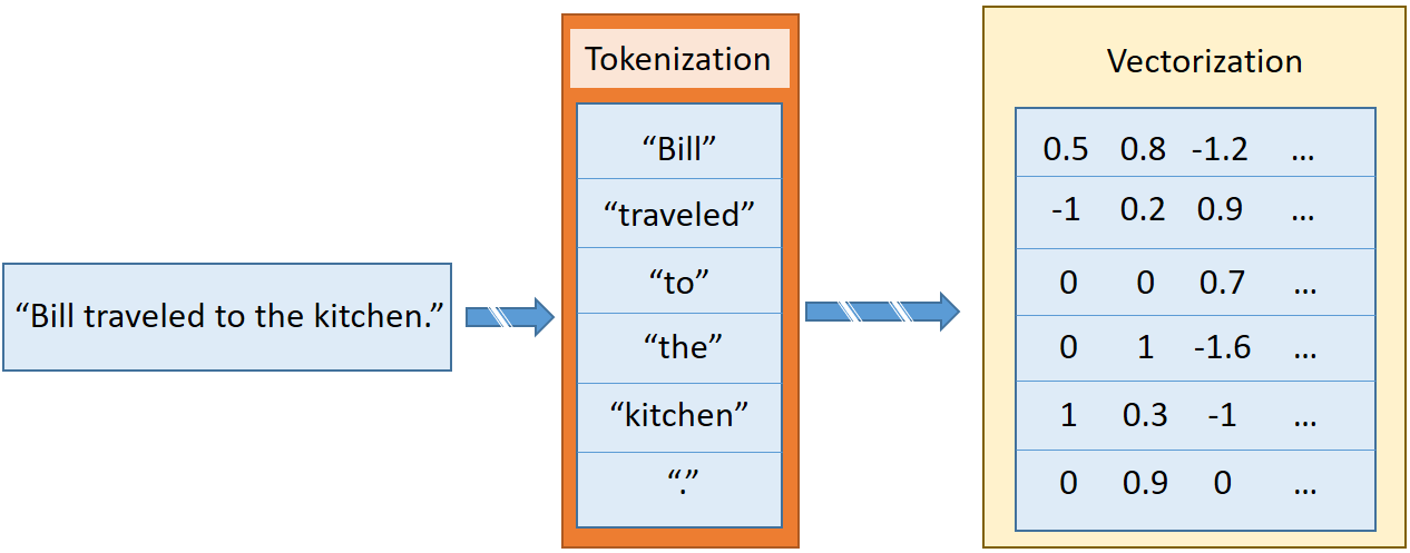
In “Textual Entailment with TensorFlow,” I discuss sentence2sequence, which is a function that would turn a string into a matrix, based on the mapping defined by GloVe. This function split up the string into tokens, which are smaller strings that are roughly equivalent to punctuation, words, or parts of words. For example, in “Bill traveled to the kitchen,” there are six tokens: five that correspond to each of the words, and the last for the period at the end. Each token gets individually vectorized, resulting in a list of vectors corresponding to each sentence, as shown in Figure 2.

In some tasks in bAbI, the system will encounter words that are not in the GloVe word vectorization. In order for the network to be capable of processing these unknown words, we need to maintain a consistent vectorization of those words. Common practice is to replace all unknown tokens with a single <UNK> vector, but this isn’t always effective. Instead, we can use randomization to draw a new vectorization for each unique unknown token.

The first time we run across a new unknown token, we simply draw a new vectorization from the (Gaussian-approximated) distribution of the original GloVe vectorizations, and add that vectorization back to the GloVe word map. To gather the distribution hyperparameters, Numpy has functions that automatically calculate variance and mean.

fill_unk will take care of giving us a new word vectorization whenever we need one.

# Deserialize GloVe vectors
glove_wordmap = {}
with open(glove_vectors_file, "r", encoding="utf8") as glove:
    for line in glove:
        name, vector = tuple(line.split(" ", 1))
        glove_wordmap[name] = np.fromstring(vector, sep=" ")

wvecs = []
for item in glove_wordmap.items():
    wvecs.append(item[1])
s = np.vstack(wvecs)

# Gather the distribution hyperparameters
v = np.var(s,0) 
m = np.mean(s,0) 
RS = np.random.RandomState()

def fill_unk(unk):
    global glove_wordmap
    glove_wordmap[unk] = RS.multivariate_normal(m,np.diag(v))
    return glove_wordmap[unk]

Known or unknown

The limited vocabulary of bAbI tasks means the network can learn the relationships between words even without knowing what the words mean. However, for speed of learning, we should choose vectorizations that have inherent meaning when we can. To do this, we use a greedy search for words that exist in Stanford’s GLoVe word vectorization data set, and if the word does not exist, then we fill in the entire word with an unknown, randomly created, new representation.

Under that model of word vectorization, we can define a new sentence2sequence:

def sentence2sequence(sentence):
    """

    - Turns an input paragraph into an (m,d) matrix, 
        where n is the number of tokens in the sentence
        and d is the number of dimensions each word vector has.

      TensorFlow doesn't need to be used here, as simply
      turning the sentence into a sequence based off our 
      mapping does not need the computational power that
      TensorFlow provides. Normal Python suffices for this task.
    """
    tokens = sentence.strip('"(),-').lower().split(" ")
    rows = []
    words = []
    #Greedy search for tokens
    for token in tokens:
        i = len(token)
        while len(token) > 0:
            word = token[:i]
            if word in glove_wordmap:
                rows.append(glove_wordmap[word])
                words.append(word)
                token = token[i:]
                i = len(token)
                continue
            else:
                i = i-1
            if i == 0:
                # word OOV
                # https://arxiv.org/pdf/1611.01436.pdf
                rows.append(fill_unk(token))
                words.append(token)
                break
    return np.array(rows), words

Now we can package all the data together needed for each question, including the vectorization of the contexts, questions, and answers. In bAbI, contexts are defined by a numbered sequence of sentences, which contextualize deserializes into a list of sentences associated with one context. Questions and answers are on the same line, separated by tabs, so we can use tabs as a marker of whether a specific line refers to a question or not. When the numbering resets, future questions will refer to the new context (note that often there is more than one question corresponding to a single context). Answers also contain one other piece of information that we keep but don’t need to use: the number(s) corresponding to the sentences needed to answer the question, in the reference order. In our system, the network will teach itself which sentences are needed to answer the question.

def contextualize(set_file):
    """
    Read in the dataset of questions and build question+answer -> context sets.
    Output is a list of data points, each of which is a 7-element tuple containing:
        The sentences in the context in vectorized form.
        The sentences in the context as a list of string tokens.
        The question in vectorized form.
        The question as a list of string tokens.
        The answer in vectorized form.
        The answer as a list of string tokens.
        A list of numbers for supporting statements, which is currently unused.
    """
    data = []
    context = []
    with open(set_file, "r", encoding="utf8") as train:
        for line in train:
            l, ine = tuple(line.split(" ", 1))
            # Split the line numbers from the sentences they refer to.
            if l is "1":
                # New contexts always start with 1, 
                # so this is a signal to reset the context.
                context = []
            if "\t" in ine: 
                # Tabs are the separator between questions and answers,
                # and are not present in context statements.
                question, answer, support = tuple(ine.split("\t"))
                data.append((tuple(zip(*context))+
                             sentence2sequence(question)+
                             sentence2sequence(answer)+
                             ([int(s) for s in support.split()],)))
                # Multiple questions may refer to the same context, so we don't reset it.
            else:
                # Context sentence.
                context.append(sentence2sequence(ine[:-1]))
    return data
train_data = contextualize(train_set_post_file)
test_data = contextualize(test_set_post_file)

final_train_data = []
def finalize(data):
    """
    Prepares data generated by contextualize() for use in the network.
    """
    final_data = []
    for cqas in train_data:
        contextvs, contextws, qvs, qws, avs, aws, spt = cqas

        lengths = itertools.accumulate(len(cvec) for cvec in contextvs)
        context_vec = np.concatenate(contextvs)
        context_words = sum(contextws,[])

        # Location markers for the beginnings of new sentences.
        sentence_ends = np.array(list(lengths)) 
        final_data.append((context_vec, sentence_ends, qvs, spt, context_words, cqas, avs, aws))
    return np.array(final_data)
final_train_data = finalize(train_data)   
final_test_data = finalize(test_data)

Defining hyperparameters

At this point, we have fully prepared our training data and our testing data. The next task is to construct the network we’ll use to understand the data. Let’s start by clearing out the TensorFlow default graph so we always have the option to run the network again if we want to change something.

tf.reset_default_graph()

Since this is the beginning of the actual network, let’s also define all the constants we’ll need for the network. We call these “hyperparameters,” as they define how the network looks and trains:

# Hyperparameters

# The number of dimensions used to store data passed between recurrent layers in the network.
recurrent_cell_size = 128

# The number of dimensions in our word vectorizations.
D = 50 

# How quickly the network learns. Too high, and we may run into numeric instability 
# or other issues.
learning_rate = 0.005

# Dropout probabilities. For a description of dropout and what these probabilities are, 
# see Entailment with TensorFlow.
input_p, output_p = 0.5, 0.5

# How many questions we train on at a time.
batch_size = 128

# Number of passes in episodic memory. We'll get to this later.
passes = 4

# Feed Forward layer sizes: the number of dimensions used to store data passed from feed-forward layers.
ff_hidden_size = 256

weight_decay = 0.00000001
# The strength of our regularization. Increase to encourage sparsity in episodic memory, 
# but makes training slower. Don't make this larger than leraning_rate.

training_iterations_count = 400000
# How many questions the network trains on each time it is trained. 
# Some questions are counted multiple times.

display_step = 100
# How many iterations of training occur before each validation check.

Network structure

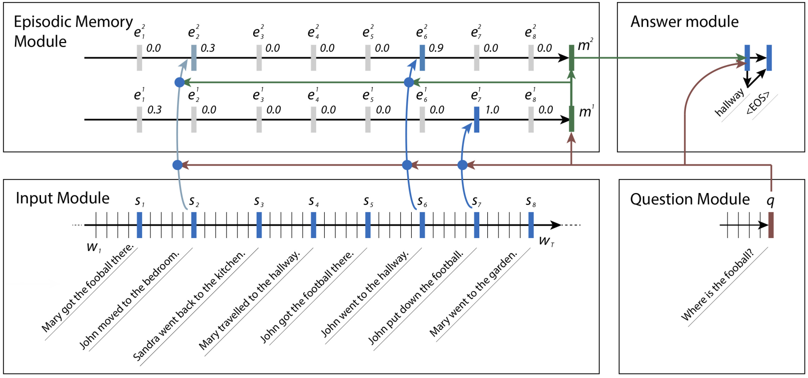
With the hyperparameters out of the way, let’s describe the network structure. The structure of this network is split loosely into four modules and is described in Ask Me Anything: Dynamic Memory Networks for Natural Language Processing.

The network is designed around having a recurrent layer’s memory be set dynamically, based on other information in the text, hence the name dynamic memory network (DMN). DMNs are loosely based on an understanding of how a human tries to answer a reading-comprehension-type question. The person gets a chance, first of all, to read the context and create memories of the facts inside. With those facts in mind, they then read the question, and re-examine the context specifically searching for the answer to that question, comparing the question to each of the facts.

Sometimes, one fact guides us to another. In the bAbI data set, the network might want to find the location of a football. It might search for sentences about the football to find that John was the last person to touch the football, then search for sentences about John to find that John had been in both the bedroom and the hallway. Once it realizes that John had been last in the hallway, it can then answer the question and confidently say that the football is in the hallway.

# Input Module

# Context: A [batch_size, maximum_context_length, word_vectorization_dimensions] tensor 
# that contains all the context information.
context = tf.placeholder(tf.float32, [None, None, D], "context")  
context_placeholder = context # I use context as a variable name later on

# input_sentence_endings: A [batch_size, maximum_sentence_count, 2] tensor that 
# contains the locations of the ends of sentences. 
input_sentence_endings = tf.placeholder(tf.int32, [None, None, 2], "sentence")

# recurrent_cell_size: the number of hidden units in recurrent layers.
input_gru = tf.contrib.rnn.GRUCell(recurrent_cell_size)

# input_p: The probability of maintaining a specific hidden input unit.
# Likewise, output_p is the probability of maintaining a specific hidden output unit.
gru_drop = tf.contrib.rnn.DropoutWrapper(input_gru, input_p, output_p)

# dynamic_rnn also returns the final internal state. We don't need that, and can
# ignore the corresponding output (_). 
input_module_outputs, _ = tf.nn.dynamic_rnn(gru_drop, context, dtype=tf.float32, scope = "input_module")

# cs: the facts gathered from the context.
cs = tf.gather_nd(input_module_outputs, input_sentence_endings)
# to use every word as a fact, useful for tasks with one-sentence contexts
s = input_module_outputs

# Question Module

# query: A [batch_size, maximum_question_length, word_vectorization_dimensions] tensor 
#  that contains all of the questions.

query = tf.placeholder(tf.float32, [None, None, D], "query")

# input_query_lengths: A [batch_size, 2] tensor that contains question length information. 
# input_query_lengths[:,1] has the actual lengths; input_query_lengths[:,0] is a simple range() 
# so that it plays nice with gather_nd.
input_query_lengths = tf.placeholder(tf.int32, [None, 2], "query_lengths")

question_module_outputs, _ = tf.nn.dynamic_rnn(gru_drop, query, dtype=tf.float32, 
                                               scope = tf.VariableScope(True, "input_module"))

# q: the question states. A [batch_size, recurrent_cell_size] tensor.
q = tf.gather_nd(question_module_outputs, input_query_lengths)

# Episodic Memory

# make sure the current memory (i.e. the question vector) is broadcasted along the facts dimension
size = tf.stack([tf.constant(1),tf.shape(cs)[1], tf.constant(1)])
re_q = tf.tile(tf.reshape(q,[-1,1,recurrent_cell_size]),size)


# Final output for attention, needs to be 1 in order to create a mask
output_size = 1 

# Weights and biases
attend_init = tf.random_normal_initializer(stddev=0.1)
w_1 = tf.get_variable("attend_w1", [1,recurrent_cell_size*7, recurrent_cell_size], 
                      tf.float32, initializer = attend_init)
w_2 = tf.get_variable("attend_w2", [1,recurrent_cell_size, output_size], 
                      tf.float32, initializer = attend_init)

b_1 = tf.get_variable("attend_b1", [1, recurrent_cell_size], 
                      tf.float32, initializer = attend_init)
b_2 = tf.get_variable("attend_b2", [1, output_size], 
                      tf.float32, initializer = attend_init)

# Regulate all the weights and biases
tf.add_to_collection(tf.GraphKeys.REGULARIZATION_LOSSES, tf.nn.l2_loss(w_1))
tf.add_to_collection(tf.GraphKeys.REGULARIZATION_LOSSES, tf.nn.l2_loss(b_1))
tf.add_to_collection(tf.GraphKeys.REGULARIZATION_LOSSES, tf.nn.l2_loss(w_2))
tf.add_to_collection(tf.GraphKeys.REGULARIZATION_LOSSES, tf.nn.l2_loss(b_2))

def attention(c, mem, existing_facts):
    """
    Custom attention mechanism.
    c: A [batch_size, maximum_sentence_count, recurrent_cell_size] tensor 
        that contains all the facts from the contexts.
    mem: A [batch_size, maximum_sentence_count, recurrent_cell_size] tensor that 
        contains the current memory. It should be the same memory for all facts for accurate results.
    existing_facts: A [batch_size, maximum_sentence_count, 1] tensor that 
        acts as a binary mask for which facts exist and which do not.

    """
    with tf.variable_scope("attending") as scope:
        # attending: The metrics by which we decide what to attend to.
        attending = tf.concat([c, mem, re_q, c * re_q,  c * mem, (c-re_q)**2, (c-mem)**2], 2)

        # m1: First layer of multiplied weights for the feed-forward network. 
        #     We tile the weights in order to manually broadcast, since tf.matmul does not
        #     automatically broadcast batch matrix multiplication as of TensorFlow 1.2.
        m1 = tf.matmul(attending * existing_facts, 
                       tf.tile(w_1, tf.stack([tf.shape(attending)[0],1,1]))) * existing_facts
        # bias_1: A masked version of the first feed-forward layer's bias
        #     over only existing facts.

        bias_1 = b_1 * existing_facts

        # tnhan: First nonlinearity. In the original paper, this is a tanh nonlinearity; 
        #        choosing relu was a design choice intended to avoid issues with 
        #        low gradient magnitude when the tanh returned values close to 1 or -1. 
        tnhan = tf.nn.relu(m1 + bias_1)

        # m2: Second layer of multiplied weights for the feed-forward network. 
        #     Still tiling weights for the same reason described in m1's comments.
        m2 = tf.matmul(tnhan, tf.tile(w_2, tf.stack([tf.shape(attending)[0],1,1])))

        # bias_2: A masked version of the second feed-forward layer's bias.
        bias_2 = b_2 * existing_facts

        # norm_m2: A normalized version of the second layer of weights, which is used 
        #     to help make sure the softmax nonlinearity doesn't saturate.
        norm_m2 = tf.nn.l2_normalize(m2 + bias_2, -1)

        # softmaxable: A hack in order to use sparse_softmax on an otherwise dense tensor. 
        #     We make norm_m2 a sparse tensor, then make it dense again after the operation.
        softmax_idx = tf.where(tf.not_equal(norm_m2, 0))[:,:-1]
        softmax_gather = tf.gather_nd(norm_m2[...,0], softmax_idx)
        softmax_shape = tf.shape(norm_m2, out_type=tf.int64)[:-1]
        softmaxable = tf.SparseTensor(softmax_idx, softmax_gather, softmax_shape)
        return tf.expand_dims(tf.sparse_tensor_to_dense(tf.sparse_softmax(softmaxable)),-1)

# facts_0s: a [batch_size, max_facts_length, 1] tensor 
#     whose values are 1 if the corresponding fact exists and 0 if not.
facts_0s = tf.cast(tf.count_nonzero(input_sentence_endings[:,:,-1:],-1,keep_dims=True),tf.float32)


with tf.variable_scope("Episodes") as scope:
    attention_gru = tf.contrib.rnn.GRUCell(recurrent_cell_size)

    # memory: A list of all tensors that are the (current or past) memory state 
    #   of the attention mechanism.
    memory = [q]

    # attends: A list of all tensors that represent what the network attends to.
    attends = []
    for a in range(passes):
        # attention mask
        attend_to = attention(cs, tf.tile(tf.reshape(memory[-1],[-1,1,recurrent_cell_size]),size),
                              facts_0s)

        # Inverse attention mask, for what's retained in the state.
        retain = 1-attend_to

        # GRU pass over the facts, according to the attention mask.
        while_valid_index = (lambda state, index: index < tf.shape(cs)[1])
        update_state = (lambda state, index: (attend_to[:,index,:] * 
                                                 attention_gru(cs[:,index,:], state)[0] + 
                                                 retain[:,index,:] * state))
        # start loop with most recent memory and at the first index
        memory.append(tuple(tf.while_loop(while_valid_index,
                          (lambda state, index: (update_state(state,index),index+1)),
                           loop_vars = [memory[-1], 0]))[0]) 

        attends.append(attend_to)

        # Reuse variables so the GRU pass uses the same variables every pass.
        scope.reuse_variables()

# Answer Module

# a0: Final memory state. (Input to answer module)
a0 = tf.concat([memory[-1], q], -1)

# fc_init: Initializer for the final fully connected layer's weights.
fc_init = tf.random_normal_initializer(stddev=0.1) 

with tf.variable_scope("answer"):
    # w_answer: The final fully connected layer's weights.
    w_answer = tf.get_variable("weight", [recurrent_cell_size*2, D], 
                               tf.float32, initializer = fc_init)
    # Regulate the fully connected layer's weights
    tf.add_to_collection(tf.GraphKeys.REGULARIZATION_LOSSES, 
                     tf.nn.l2_loss(w_answer)) 

    # The regressed word. This isn't an actual word yet; 
    #    we still have to find the closest match.
    logit = tf.expand_dims(tf.matmul(a0, w_answer),1)

    # Make a mask over which words exist.
    with tf.variable_scope("ending"):
        all_ends = tf.reshape(input_sentence_endings, [-1,2])
        range_ends = tf.range(tf.shape(all_ends)[0])
        ends_indices = tf.stack([all_ends[:,0],range_ends], axis=1)
        ind = tf.reduce_max(tf.scatter_nd(ends_indices, all_ends[:,1],
                                          [tf.shape(q)[0], tf.shape(all_ends)[0]]),
                            axis=-1)
        range_ind = tf.range(tf.shape(ind)[0])
        mask_ends = tf.cast(tf.scatter_nd(tf.stack([ind, range_ind], axis=1), 
                                          tf.ones_like(range_ind), [tf.reduce_max(ind)+1, 
                                                                    tf.shape(ind)[0]]), bool)
        # A bit of a trick. With the locations of the ends of the mask (the last periods in 
        #  each of the contexts) as 1 and the rest as 0, we can scan with exclusive or 
        #  (starting from all 1). For each context in the batch, this will result in 1s 
        #  up until the marker (the location of that last period) and 0s afterwards.
        mask = tf.scan(tf.logical_xor,mask_ends, tf.ones_like(range_ind, dtype=bool))

    # We score each possible word inversely with their Euclidean distance to the regressed word.
    #  The highest score (lowest distance) will correspond to the selected word.
    logits = -tf.reduce_sum(tf.square(context*tf.transpose(tf.expand_dims(
                    tf.cast(mask, tf.float32),-1),[1,0,2]) - logit), axis=-1)

Optimizing optimization

Gradient descent is the default optimizer for a neural network. Its goal is to decrease the network’s “loss,” which is a measure of how poorly the network performs. It does this by finding the derivative of loss with respect to each of the weights under the current input, and then “descends” the weights so they’ll reduce the loss. Most of the time, this works well enough, but often it’s not ideal. There are various schemes that use “momentum” or other approximations of the more direct path to the optimal weights. One of the most useful of these optimization schemes is known as adaptive moment estimation, or Adam.

Adam estimates the first two moments of the gradient by calculating an exponentially decaying average of past iterations’ gradients and squared gradients, which correspond to the estimated mean and the estimated variance of these gradients. The calculations use two additional hyperparameters to indicate how quickly the averages decay with the addition of new information. The averages are initialized as zero, which leads to bias toward zero, especially when those hyperparameters near one.

In order to counteract that bias, Adam computes bias-corrected moment estimates that are greater in magnitude than the originals. The corrected estimates are then used to update the weights throughout the network. The combination of these estimates make Adam one of the best choices overall for optimization, especially for complex networks. This applies doubly to data that is very sparse, such as is common in natural language processing tasks.

In TensorFlow, we can use Adam by creating a tf.train.AdamOptimizer.

# Training

# gold_standard: The real answers.
gold_standard = tf.placeholder(tf.float32, [None, 1, D], "answer")
with tf.variable_scope('accuracy'):
    eq = tf.equal(context, gold_standard)
    corrbool = tf.reduce_all(eq,-1)
    logloc = tf.reduce_max(logits, -1, keep_dims = True)
    # locs: A boolean tensor that indicates where the score 
    #  matches the minimum score. This happens on multiple dimensions, 
    #  so in the off chance there's one or two indexes that match 
    #  we make sure it matches in all indexes.
    locs = tf.equal(logits, logloc)

    # correctsbool: A boolean tensor that indicates for which 
    #   words in the context the score always matches the minimum score.
    correctsbool = tf.reduce_any(tf.logical_and(locs, corrbool), -1)
    # corrects: A tensor that is simply correctsbool cast to floats.
    corrects = tf.where(correctsbool, tf.ones_like(correctsbool, dtype=tf.float32), 
                        tf.zeros_like(correctsbool,dtype=tf.float32))

    # corr: corrects, but for the right answer instead of our selected answer.
    corr = tf.where(corrbool, tf.ones_like(corrbool, dtype=tf.float32), 
                        tf.zeros_like(corrbool,dtype=tf.float32))
with tf.variable_scope("loss"):
    # Use sigmoid cross entropy as the base loss, 
    #  with our distances as the relative probabilities. There are
    #  multiple correct labels, for each location of the answer word within the context.
    loss = tf.nn.sigmoid_cross_entropy_with_logits(logits = tf.nn.l2_normalize(logits,-1),
                                                   labels = corr)

    # Add regularization losses, weighted by weight_decay.
    total_loss = tf.reduce_mean(loss) + weight_decay * tf.add_n(
        tf.get_collection(tf.GraphKeys.REGULARIZATION_LOSSES))

# TensorFlow's default implementation of the Adam optimizer works. We can adjust more than 
#  just the learning rate, but it's not necessary to find a very good optimum.
optimizer = tf.train.AdamOptimizer(learning_rate)

# Once we have an optimizer, we ask it to minimize the loss 
#   in order to work towards the proper training.
opt_op = optimizer.minimize(total_loss)

# Initialize variables
init = tf.global_variables_initializer()

# Launch the TensorFlow session
sess = tf.Session()
sess.run(init)

Train the network

With everything set and ready, we can begin batching our training data to train our network! While the system is training, we should check on how well the network is doing in terms of accuracy. We do this with a validation set, which is taken from testing data so it has no overlap with the training data.

Using a validation set based on testing data allows us to get a better sense of how well the network can generalize what it learns and apply it to other contexts. If we validate on the training data, the network may overfit—in other words, learn specific examples and memorize the answers to them, which doesn’t help the network answer new questions.

If you installed TQDM, you can use it to keep track of how long the network has been training and receive an estimate of when training will finish. You can stop the training at any time if you feel the results are good enough by interrupting the Jupyter Notebook kernel.

def prep_batch(batch_data, more_data = False):
    """
        Prepare all the preproccessing that needs to be done on a batch-by-batch basis.
    """
    context_vec, sentence_ends, questionvs, spt, context_words, cqas, answervs, _ = zip(*batch_data)
    ends = list(sentence_ends)
    maxend = max(map(len, ends))
    aends = np.zeros((len(ends), maxend))
    for index, i in enumerate(ends):
        for indexj, x in enumerate(i):
            aends[index, indexj] = x-1
    new_ends = np.zeros(aends.shape+(2,))

    for index, x in np.ndenumerate(aends):
        new_ends[index+(0,)] = index[0]
        new_ends[index+(1,)] = x

    contexts = list(context_vec)
    max_context_length = max([len(x) for x in contexts])
    contextsize = list(np.array(contexts[0]).shape)
    contextsize[0] = max_context_length
    final_contexts = np.zeros([len(contexts)]+contextsize)

    contexts = [np.array(x) for x in contexts]
    for i, context in enumerate(contexts):
        final_contexts[i,0:len(context),:] = context
    max_query_length = max(len(x) for x in questionvs)
    querysize = list(np.array(questionvs[0]).shape)
    querysize[:1] = [len(questionvs),max_query_length]
    queries = np.zeros(querysize)
    querylengths = np.array(list(zip(range(len(questionvs)),[len(q)-1 for q in questionvs])))
    questions = [np.array(q) for q in questionvs]
    for i, question in enumerate(questions):
        queries[i,0:len(question),:] = question
    data = {context_placeholder: final_contexts, input_sentence_endings: new_ends, 
                            query:queries, input_query_lengths:querylengths, gold_standard: answervs}
    return (data, context_words, cqas) if more_data else data

# Use TQDM if installed
tqdm_installed = False
try:
    from tqdm import tqdm
    tqdm_installed = True
except:
    pass


# Prepare validation set
batch = np.random.randint(final_test_data.shape[0], size=batch_size*10)
batch_data = final_test_data[batch]

validation_set, val_context_words, val_cqas = prep_batch(batch_data, True)

# training_iterations_count: The number of data pieces to train on in total
# batch_size: The number of data pieces per batch
def train(iterations, batch_size):
    training_iterations = range(0,iterations,batch_size)
    if tqdm_installed:
        # Add a progress bar if TQDM is installed
        training_iterations = tqdm(training_iterations)

    wordz = []
    for j in training_iterations:

        batch = np.random.randint(final_train_data.shape[0], size=batch_size)
        batch_data = final_train_data[batch]

        sess.run([opt_op], feed_dict=prep_batch(batch_data))
        if (j/batch_size) % display_step == 0:

            # Calculate batch accuracy
            acc, ccs, tmp_loss, log, con, cor, loc  = sess.run([corrects, cs, total_loss, logit,
                                                                context_placeholder,corr, locs], 
                                                               feed_dict=validation_set)
            # Display results
            print("Iter " + str(j/batch_size) + ", Minibatch Loss= ",tmp_loss,
                  "Accuracy= ", np.mean(acc))
train(30000,batch_size) # Small amount of training for preliminary results

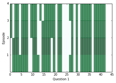
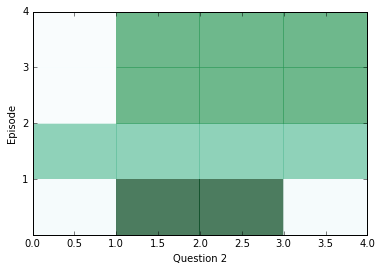
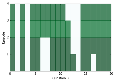
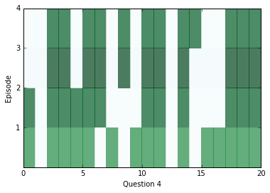
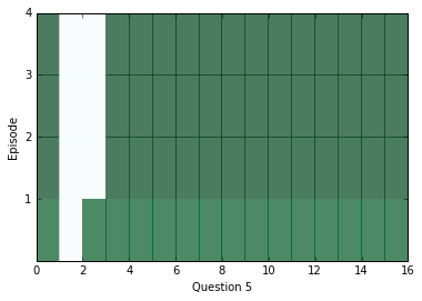
After a little bit of training, let’s peek inside and see what kinds of answers we’re getting from the network. In the diagrams below, we visualize attention over each of the episodes (rows) for all the sentences (columns) in our context; darker colors represent more attention paid to that sentence on that episode.

You should see attention change between at least two episodes for each question, but sometimes attention will be able to find the answer within one, and sometimes it will take all four episodes. If the attention appears to be blank, it may be saturating and paying attention to everything at once. In that case, you can try training with a higher weight_decay in order to discourage that from happening. Later on in training, saturation becomes extremely common.

ancr = sess.run([corrbool,locs, total_loss, logits, facts_0s, w_1]+attends+
                [query, cs, question_module_outputs],feed_dict=validation_set)
a = ancr[0]
n = ancr[1]
cr = ancr[2]
attenders = np.array(ancr[6:-3]) 
faq = np.sum(ancr[4], axis=(-1,-2)) # Number of facts in each context

limit = 5
for question in range(min(limit, batch_size)):
    plt.yticks(range(passes,0,-1))
    plt.ylabel("Episode")
    plt.xlabel("Question "+str(question+1))
    pltdata = attenders[:,question,:int(faq[question]),0] 
    # Display only information about facts that actually exist, all others are 0
    pltdata = (pltdata - pltdata.mean()) / ((pltdata.max() - pltdata.min() + 0.001)) * 256
    plt.pcolor(pltdata, cmap=plt.cm.BuGn, alpha=0.7)
    plt.show()

#print(list(map((lambda x: x.shape),ancr[3:])), new_ends.shape)

In order to see what the answers for the above questions were, we can use the location of our distance score in the context as an index and see what word is at that index.

# Locations of responses within contexts
indices = np.argmax(n,axis=1)

# Locations of actual answers within contexts 
indicesc = np.argmax(a,axis=1)

for i,e,cw, cqa in list(zip(indices, indicesc, val_context_words, val_cqas))[:limit]:
    ccc = " ".join(cw)
    print("TEXT: ",ccc)
    print ("QUESTION: ", " ".join(cqa[3]))
    print ("RESPONSE: ", cw[i], ["Correct", "Incorrect"][i!=e])
    print("EXPECTED: ", cw[e])
    print()

    TEXT:  mary travelled to the bedroom . mary journeyed to the bathroom . mary got the football there . mary passed the football to fred .
    QUESTION:  who received the football ?
    RESPONSE:  mary Incorrect
    EXPECTED:  fred

    TEXT:  bill grabbed the apple there . bill got the football there . jeff journeyed to the bathroom . bill handed the apple to jeff . jeff handed the apple to bill . bill handed the apple to jeff . jeff handed the apple to bill . bill handed the apple to jeff .
    QUESTION:  what did bill give to jeff ?
    RESPONSE:  apple Correct
    EXPECTED:  apple

    TEXT:  bill moved to the bathroom . mary went to the garden . mary picked up the apple there . bill moved to the kitchen . mary left the apple there . jeff got the football there . jeff went back to the kitchen . jeff gave the football to fred .
    QUESTION:  what did jeff give to fred ?
    RESPONSE:  apple Incorrect
    EXPECTED:  football

    TEXT:  jeff travelled to the bathroom . bill journeyed to the bedroom . jeff journeyed to the hallway . bill took the milk there . bill discarded the milk . mary moved to the bedroom . jeff went back to the bedroom . fred got the football there . bill grabbed the milk there . bill passed the milk to mary . mary gave the milk to bill . bill discarded the milk there . bill went to the kitchen . bill got the apple there .
    QUESTION:  who gave the milk to bill ?
    RESPONSE:  jeff Incorrect
    EXPECTED:  mary

    TEXT:  fred travelled to the bathroom . jeff went to the bathroom . mary went back to the bathroom . fred went back to the bedroom . fred moved to the office . mary went back to the bedroom . jeff got the milk there . bill journeyed to the garden . mary went back to the kitchen . fred went to the bedroom . mary journeyed to the bedroom . jeff put down the milk there . jeff picked up the milk there . bill went back to the office . mary went to the kitchen . jeff went back to the kitchen . jeff passed the milk to mary . mary gave the milk to jeff . jeff gave the milk to mary . mary got the football there . bill travelled to the bathroom . fred moved to the garden . fred got the apple there . mary handed the football to jeff . fred put down the apple . jeff left the football .
    QUESTION:  who received the football ?
    RESPONSE:  mary Incorrect
    EXPECTED:  jeff

Let’s keep training! In order to get good results, you may have to train for a long period of time (on my home desktop, it took about 12 hours), but you should eventually be able to reach very high accuracies (over 90%). Experienced users of Jupyter Notebook should note that at any time, you can interrupt training and still save the progress the network has made so far, as long as you keep the same tf.Session; this is useful if you want to visualize the attention and answers the network is currently giving.

train(training_iterations_count, batch_size)

# Final testing accuracy
print(np.mean(sess.run([corrects], feed_dict= prep_batch(final_test_data))[0]))

0.95

Once we’re done viewing what our model is returning, we can close the session to free up system resources.

sess.close()

Looking for more?

There’s a lot still left to be done and experimented with:

• Other tasks in bAbI. We’ve only sampled the many tasks that bAbI has to offer. Try changing the preprocessing to fit another task and see how our dynamic memory network performs on it. You may want to retrain the network before you try running it on the new task, of course. If the task doesn’t guarantee the answer is inside the context, you may want to compare output to a dictionary of words and their corresponding vectors instead. (Those tasks are 6-10 and 17-20.) I recommend trying task 1 or 3, which you can do by changing the values of test_set_file and train_set_file.
• Supervised training. Our attention mechanism is unsupervised, in that we don’t specify explicitly which sentences should be attended to and instead let the network figure that out on its own. Try adding loss to the network that encourages the attention mechanism toward attending to the right sentences.
• Coattention. Instead of attending simply over the input sentences, some researchers have found success in what they call “dynamic coattention networks”, which attends over a matrix representing two locations in two sequences simultaneously.
• Alternate vectorization schemes and sources. Try making more intelligent mappings between sentences and vectors, or maybe use a different data set. GloVe offers larger corpi of up to 840 billion distinct tokens, of 300 dimensions each.

This post is a collaboration between O’Reilly and TensorFlow. See our statement of editorial independence.