Build generative models using Apache MXNet
A step-by-step tutorial to build generative models through generative adversarial networks (GANs) to generate a new image from existing images.
 Spiral staircase (source: stokpic via Pixabay)
In our previous notebooks, we used a deep learning technique called convolution neural network (CNN) to classify text and images. A CNN is an example of a discriminative model, which creates a decision boundary to classify a given input signal (data) as either being in or out of a classification, such as email spam.
Deep learning models in recent times have been used to create even more powerful and useful models called generative models. A generative model doesn’t just create a decision boundary, but understands the underlying distribution of values. Using this insight, a generative model can also generate new data or classify a given input data. Here are some examples of generative models:
- Producing a new song or combining two genres of songs to create an entirely different song
- Synthesizing new images from existing images
- Upgrading images to a higher resolution in order to remove fuzziness, improve image quality, and much more
In general, generative models can be used on any form of data to learn the underlying distribution, generate new data, and augment existing data.
In this tutorial, we are going to build generative models through generative adversarial networks (GANs) to generate a new image from existing images. Our code will use Apache MXNet’s Gluon API.
By the end of the notebook, you will be able to:
- Understand generative models
- Place generative models into the context of deep neural networks
- Implement a generative adversarial network (GAN)
How generative models go further than discriminative models
Let’s see the power of generative models using a trivial example. The following depicts the heights of 10 humans and Martians.
Martian (height in centimeter):
250,260,270,300,220,260,280,290,300,310
Human (height in centimeter):
160,170,180,190,175,140,180,210,140,200
The heights of human beings follow a normal distribution, showing up as a bell-shaped curve on the a graph (see Figure 1). Martians tend to be much taller than humans, but also have a normal distribution. So, let’s input the heights of humans and Martians into both discriminative and generative models.

If we train a discriminative model, it will just plot a decision boundary (see Figure 2). The model misclassifies just one human—the accuracy is quite good overall. But the model doesn’t learn about the underlying distribution of data, so it is not suitable for building the powerful applications listed in the beginning of this article.
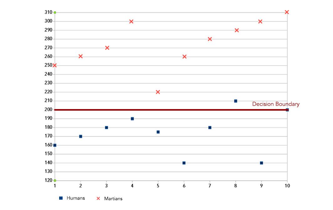
In contrast, a generative model will learn the underlying distribution (lower dimension representation) for Martian (mean=274, std=8.71) and Human (mean=174, std=7.32). If we know the normal distribution for Martians (mean=274, std=8.71), we can produce new data by generating a random number between 0 and 1 (uniform distribution) and then querying the normal distribution of Martians to get a value: say, 275 cm.
Using the underlying distribution, we can generate new Martians and humans, or a new interbreed species (humars). We have infinite ways to generate data because we can manipulate the underlying distribution of data. We can also use this model for classifying Martians and humans, just like the discriminative model. For a concrete understanding of generative versus discriminative models, please check the article “Generative and Discriminative Text Classification with Recurrent Neural Networks” by Yogatama, et al.
Examples of discriminative models include logistic regression and support vector machines (SVNs), while examples of generative models include hidden Markov models and naive Bayes classifiers.
Using discriminative and generative models in neural networks
Suppose, we want train a discriminative model called “m-dis” and a generative model called “m-gen-partial” to find the difference between a dog and a cat. The discriminative model will have a softmax layer as the final layer to do binary classification. Except for the input layer and the softmax layer, all the other layers (the hidden layers) try to learn a representation of the input (cat or dog?) that can reduce the loss at the final layer. The hidden layer may learn a rule like, “if the eyes are blue and the image has brown stripes, it is a cat, otherwise it is a dog,” ignoring other important features like the shape of the body, height, etc.
In contrast, the generative model is trained to learn a lower-dimension representation (distribution) that can represent the input image of cat or dog. The final layer is not a softmax layer for classification. The hidden layer can learn about the general features of a cat or dog (shape, color, height, etc.). Moreover, the data set needs no labeling, as we are training only to extract features to represent the input data. We can then tweak the generative model to classify an animal by adding a softmax classifier at the end and by training it with few labeled examples of cats and dogs. We can also generate new data by adding a decoder network to the model. Adding a decoder network is not trivial, and we have explained this in the “Designing the GAN network” section.
Preparing your environment
If you’re working in the AWS Cloud, you can save yourself a lot of installation work by using an Amazon SageMaker, pre-configured for deep learning. If you have done this, skip steps 1-5 below.
If you are using a Conda environment, remember to install pip inside conda by typing conda install pip after you activate an environment. This will save you a lot of problems down the road.
Here’s how to get set up:
- Install Anaconda, a package manager. It is easier to install Python libraries using Anaconda.
You can use this command:
curl -O https://repo.continuum.io/archive/Anaconda3-4.2.0-Linux-x86_64.sh
chmod +x Anaconda3-4.2.0-Linux-x86_64.sh
./Anaconda3-4.2.0-Linux-x86_64.sh - Install scikit-learn, a general-purpose scientific computing library. We’ll use this to pre-process our data. You can install it with
conda install scikit-learn. - Grab the Jupyter Notebook, with
conda install jupyter notebook. -
Get MXNet, an open source deep learning library. The Python notebook was tested on version 0.12.0 of MxNet, and you can install using pip as follows: pip install mxnet-cu90 (if you have a GPU) else use pip install mxnet –pre. Please see the documentation for details
-
After you activate the anaconda environment, type these commands in it:
source activate mxnet
The consolidated list of commands is:
curl -O https://repo.continuum.io/archive/Anaconda3-4.2.0-Linux-x86_64.sh
chmod +x Anaconda3-4.2.0-Linux-x86_64.sh
./Anaconda3-4.2.0-Linux-x86_64.sh
conda install pip
pip install opencv-python
conda install scikit-learn
conda install jupyter notebook
pip install mxnet-cu90
- You can download the MXNet notebook for this part of the tutorial, where we’ve created and run all this code, and play with it! Adjust the hyperparameters and experiment with different approaches to neural network architecture.
Generative adversarial network (GAN)
Generative adversarial network is a neural network model based on a zero-sum game from game theory. The application typically consists of two different neural networks called discriminator and generator, where each network tries to outperform the other. Let’s consider an example to understand a GAN network.
Let’s assume there is a bank (discriminator) that detects whether a given currency is real or fake using machine learning. A fraudster (generator) builds a machine learning model to counterfeit fake currency notes by looking at the real currency notes. The counterfeiter deposits the fake notes in the bank and the bank tries to identify which currencies deposited there are fake (see Figure 3).
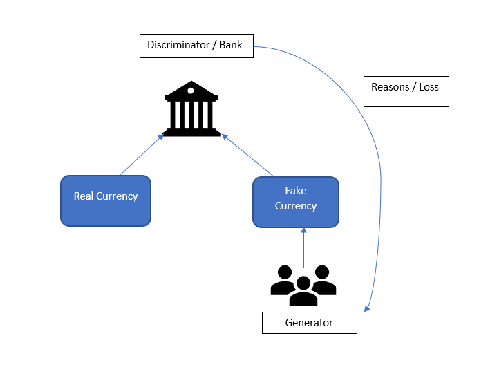
If the bank tells the fraudster why it classified these notes as fake, he can improve his model based on those reasons. After multiple iterations, the bank cannot tell the difference between the “real” and “fake” currency. This is the idea behind GANs.
So, now let’s implement a simple GAN network to generate new anime images. I encourage you to download the notebook. You are welcome to adjust the hyperparameters and experiment with different approaches to the neural network architecture.
Preparing the data set
We use a library called Brine to download our data set. Brine has many data sets, so we can choose the data set that we want to download. To install Brine and download our data set, do the following:
pip install brine-iobrine install jayleicn/anime-faces
This tutorial uses the Anime-faces data set, which contains over 100,000 anime images collected from the internet.
Once the data set is downloaded, you can load it using the following code:
# brine for loading anime-faces datasetimportbrineanime_train=brine.load_dataset('jayleicn/anime-faces')
We also need to normalize the pixel value of each image to [-1 to 1] and reshape each image from (width X height X channels) to (channels X width X height), because the latter format is what MxNet expects. The transform function does the job of reshaping the input image into the required shape expected by the MxNet model.
deftransform(data,target_wd,target_ht):# resize to target_wd * target_htdata=mx.image.imresize(data,target_wd,target_ht)# transpose from (target_wd, target_ht, 3)# to (3, target_wd, target_ht)data=nd.transpose(data,(2,0,1))# normalize to [-1, 1]data=data.astype(np.float32)/127.5-1returndata.reshape((1,)+data.shape)
The getImageList function reads the images from the training_folder and returns the images as a list, which is then transformed into an MxNet array.
# Read images, call the transform function, attach it to listdefgetImageList(base_path,training_folder):img_list=[]fortrainintraining_folder:fname=base_path+train.imageimg_arr=mx.image.imread(fname)img_arr=transform(img_arr,target_wd,target_ht)img_list.append(img_arr)returnimg_listbase_path='brine_datasets/jayleicn/anime-faces/images/'img_list=getImageList('brine_datasets/jayleicn/anime-faces/images/',training_fold)
Designing the GAN network
We now need to design the two separate networks, the discriminator and the generator. The generator takes a random vector of shape (batchsize X N), where N is an integer, and converts it to an image of shape (batchsize X channels X width X height).
The generator uses transpose convolutions to upscale the input vectors. This is very similar to how a decoder unit in an autoencoder maps a lower-dimension vector into a higher-dimensional vector representation. You can choose to design your own generator network; the only the thing you need to be careful about is the input and the output shapes. The input to the generator network should be of low dimension (we use 1×150, latent_z_size) and output should be the expected number of channels (3 for color images), width, and height (3 x width x height). Here’s the snippet of a generator network.
# simple generator. Use any models but should upscale the latent variable(randome vectors) to 64 * 64 * 3 channel imagewithnetG.name_scope():# input is random_z (batchsize X 150 X 1), going into a tranposed convolutionnetG.add(nn.Conv2DTranspose(ngf*8,4,1,0))netG.add(nn.BatchNorm())netG.add(nn.Activation('relu'))# output size. (ngf*8) x 4 x 4netG.add(nn.Conv2DTranspose(ngf*4,4,2,1))netG.add(nn.BatchNorm())netG.add(nn.Activation('relu'))# output size. (ngf*8) x 8 x 8netG.add(nn.Conv2DTranspose(ngf*2,4,2,1))netG.add(nn.BatchNorm())netG.add(nn.Activation('relu'))# output size. (ngf*8) x 16 x 16netG.add(nn.Conv2DTranspose(ngf,4,2,1))netG.add(nn.BatchNorm())netG.add(nn.Activation('relu'))# output size. (ngf*8) x 32 x 32netG.add(nn.Conv2DTranspose(nc,4,2,1))netG.add(nn.Activation('tanh'))# use tanh , we need an output that is between -1 to 1, not 0 to 1# Rememeber the input image is normalised between -1 to 1, so should be the output# output size. (nc) x 64 x 64
Our discriminator is a binary image classification network that maps the image of shape (batchsize X channels X width x height) into a lower-dimension vector of shape (batchsize X 1). Again, you can use any model that does binary classification with reasonable accuracy.
Here’s the snippet of the discriminator network:
withnetD.name_scope():# input is (nc) x 64 x 64netD.add(nn.Conv2D(ndf,4,2,1))netD.add(nn.LeakyReLU(0.2))# output size. (ndf) x 32 x 32netD.add(nn.Conv2D(ndf*2,4,2,1))netD.add(nn.BatchNorm())netD.add(nn.LeakyReLU(0.2))# output size. (ndf) x 16 x 16netD.add(nn.Conv2D(ndf*4,4,2,1))netD.add(nn.BatchNorm())netD.add(nn.LeakyReLU(0.2))# output size. (ndf) x 8 x 8netD.add(nn.Conv2D(ndf*8,4,2,1))netD.add(nn.BatchNorm())netD.add(nn.LeakyReLU(0.2))# output size. (ndf) x 4 x 4netD.add(nn.Conv2D(1,4,1,0))
Training the GAN network
The training of a GAN network is not straightforward, but it is simple. Figure 4 illustrates the training process.
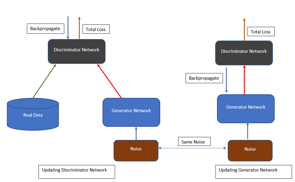
The real images are given a label of 1, and the fake images are given a label of 0.
# real label is the labels of real imagereal_label=nd.ones((batch_size,),ctx=ctx)# fake labels is label associated with fake imagefake_label=nd.zeros((batch_size,),ctx=ctx)
Training the discriminator
A real image is now passed to the discriminator to determine whether it is real or fake, and the loss associated with the prediction is calculated as errD_real.
# train with real imageoutput=netD(data).reshape((-1,1))# The loss is a real valued numbererrD_real=loss(output,real_label)
In the next step, a random noise random_z is passed to the generator network to produce a random image. This image is then passed to the discriminator to classify it as real (1) or fake (0), thereby creating a loss, errD_fake. This errD_fake is high if the discriminator wrongly classifies the fake image (label 0) as a true image (label 1). This errD_fake is back propagated to train the discriminator to classify the fake image as a fake image (label 0). This helps the discriminator improve its accuracy.
trainwithfakeimage,seethewhatthediscriminatorpredicts# creates fake imgefake=netG(random_z)# pass it to discriminatoroutput=netD(fake.detach()).reshape((-1,1))errD_fake=loss(output,fake_label)
The total error is back propagated to tune the weights of the discriminator.
# compute the total error for fake image and the real imageerrD=errD_real+errD_fake# improve the discriminator skill by back propagating the errorerrD.backward()
Training the generator
The random noise (random_z) vector used for training the discriminator is used again to generate a fake image. We then pass the fake image to the discriminator network to obtain the classification output, and the loss is calculated. The loss is high if the fake image generated (label = 0) is not similar to the real image (label 1)—i.e., if the generator is not able to produce a fake image that can trick the discriminator to classify it as a real image (label =1). The loss is then used to fine-tune the generator network.
fake=netG(random_z)output=netD(fake).reshape((-1,1))errG=loss(output,real_label)errG.backward()
Generating new fake images
The model weights are available here. You can download the model parameters and load it using the model.load_params function.
We can use the generator network to create new fake images by providing 150 random dimensions as an input to the network (see Figure 5).
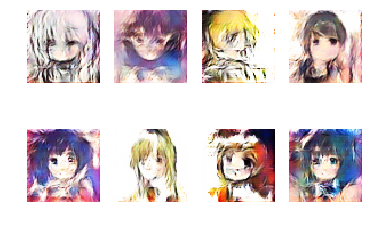
# Let's generate some random imagesnum_image=8foriinrange(num_image):# random input for the generating imagesrandom_z=mx.nd.random_normal(0,1,shape=(1,latent_z_size,1,1),ctx=ctx)img=netG(random_z)plt.subplot(2,4,i+1)visualize(img[0])plt.show()
Although the images generated look similar to the input data set, they are fuzzy. There are several other GAN networks that you can experiment with and achieve amazing results.
Conclusion
Generative models open up new opportunities for deep learning. This article has explored some of the famous generative models for image data. We learned about GAN models, which combine discriminative and generative models, and used one to generate new images very close to the input data (anime characters).
This post is a collaboration between O’Reilly and Amazon. See our statement of editorial independence.
