Deep convolutional generative adversarial networks with TensorFlow

The concept of generative adversarial networks (GANs) was introduced less than four years ago by Ian Goodfellow. Goodfellow uses the metaphor of an art critic and an artist to describe the two models—discriminators and generators—that make up GANs. An art critic (the discriminator) looks at an image and tries to determine if its real or a forgery. An artist (the generator) who wants to fool the art critic tries to make a forged image that looks as realistic as possible. These two models “battle” each other; the discriminator uses the output of the generator as training data, and the generator gets feedback from the discriminator. Each model becomes stronger in the process. In this way, GANs are able to generate new complex data, based on some amount of known input data, in this case, images.

It may sound scary to implement GANs, but it doesn’t have to be. In this tutorial, we will use TensorFlow to build a GAN that is able to generate images of human faces.

Architecture of our DCGAN

In this tutorial, we are not trying to mimic simple numerical data—we are trying to mimic an image, which should even be able to fool a human. The generator takes a randomly generated noise vector as input data and then uses a technique called deconvolution to transform the data into an image.

The discriminator is a classical convolutional neural network, which classifies real and fake images.

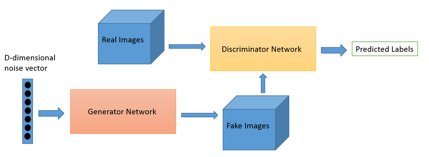
We are going to use the original DCGAN architecture from the paper Unsupervised Representation Learning with Deep Convolutional Generative Adversarial Networks, which consists of four convolutional layers for the discriminator and four deconvolutional layers for the generator.

Setup

Please access the code and Jupyter Notebook for this tutorial on GitHub. All instructions are in the README file in the GitHub repository. A helper function will automatically download the CelebA data set to get you up and running quickly. Be sure to have matplotlib installed to actually see the images and requests to download the data set. If you don’t want to install it yourself, there is a Docker image included in the repository.

The CelebA data set

The CelebFaces Attributes data set contains more than 200,000 celebrity images, each with 40 attribute annotations. Since we just want to generate images of random faces, we are going to ignore the annotations. The data set includes more than 10,000 different identities, which is perfect for our cause.

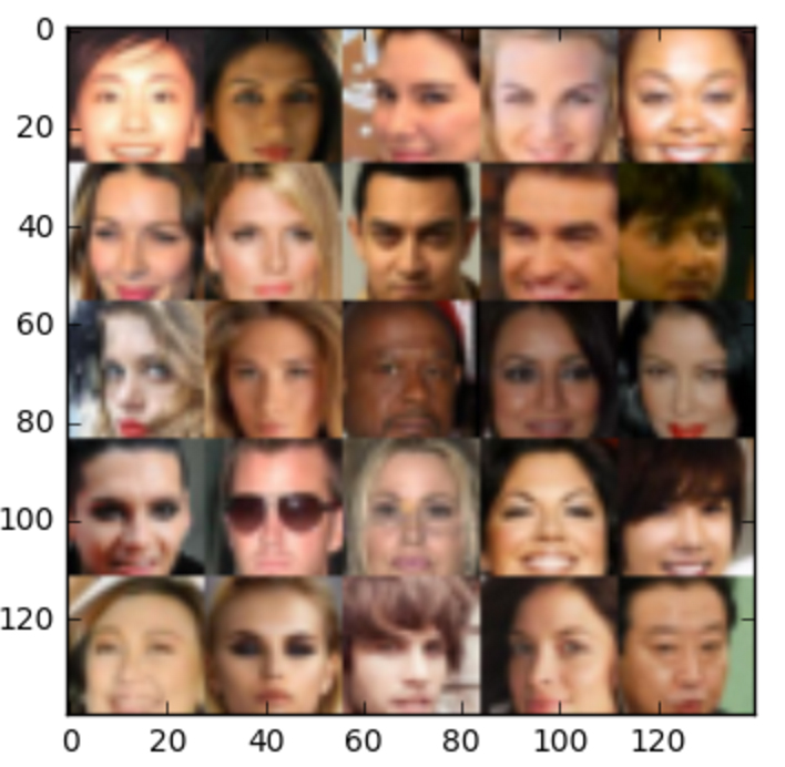
At this point, we are also going to define a function for batch generation. This function will load our images and give us an array of images according to a batch size we are going to set later. To get better results, we will crop the images, so that only the faces are showing. We will also normalize the images so that their pixel values are in a range from -0.5 to +0.5. Last, we are going to downscale the images to 28×28 after that. This makes us lose some image quality, but it decreases the training time dramatically.

Defining network input

Before we can start defining our two networks, we are going to define our inputs. We are doing this to not clutter the training function any more than it already is. Here, we are simply defining TensorFlow Placeholders for our real and fake inputs, and for the learning rate.

    inputs_real = tf.placeholder(tf.float32, shape=(None, image_width, image_height, image_channels), name='input_real')
    inputs_z = tf.placeholder(tf.float32, (None, z_dim), name='input_z')
    learning_rate = tf.placeholder(tf.float32, name='learning_rate')
   
    return inputs_real, inputs_z, learning_rate

TensorFlow makes it particularly easy to assign variables to placeholders. After we’ve done this, we can use the placeholders in our network by specifying a feed dictionary later.

The discriminator network

Finally, we are coming to the first of the dueling networks. The discriminator is the “art critic,” who tries to distinguish between real and fake images. Simply said, this is a convolutional neural network for image classification. If you already have some experience with deep learning, chances are you have already built a network very similar to this one.

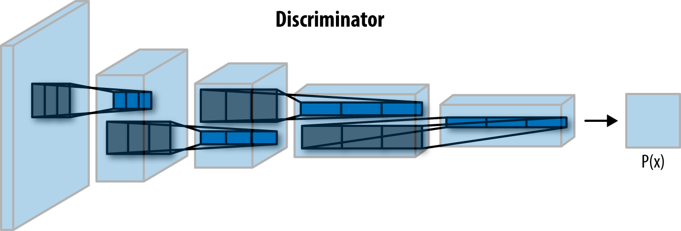
We are going to use a TensorFlow variable scope when defining this network. This helps us in the training process later so we can reuse our variable names for both the discriminator and the generator.

def discriminator(images, reuse=False):
    """
    Create the discriminator network
    """
   
    with tf.variable_scope('discriminator', reuse=reuse):
        # … the model

The discriminator network consists of three convolutional layers, opposed to four like in the original architecture. We remove this last layer to simplify the model a little bit. This way, the training goes a lot faster without losing too much quality.This makes training go a little bit faster. For every layer of the network, we are going to perform a convolution, then we are going to perform batch normalization to make the network faster and more accurate, and, finally, we are going to perform a Leaky ReLu to further speed up the training. At the end, we flatten the output of the last layer and use the sigmoid activation function to get a classification. We now have a prediction whether the image is real or not.

The generator network

The generator goes the other way: It is the “artist” who is trying to fool the discriminator. The generator makes use of deconvolutional layers. They are the exact opposite of a convolutional layers: Instead of performing convolutions until the image is transformed into simple numerical data, such as a classification, we perform deconvolutions to transform numerical data into an image. This is a concept which is not as known as a simple convolutional layer, since it’s used for advanced topics. We are wrapping this in a variable scope as well, just as we did in the discriminator network.

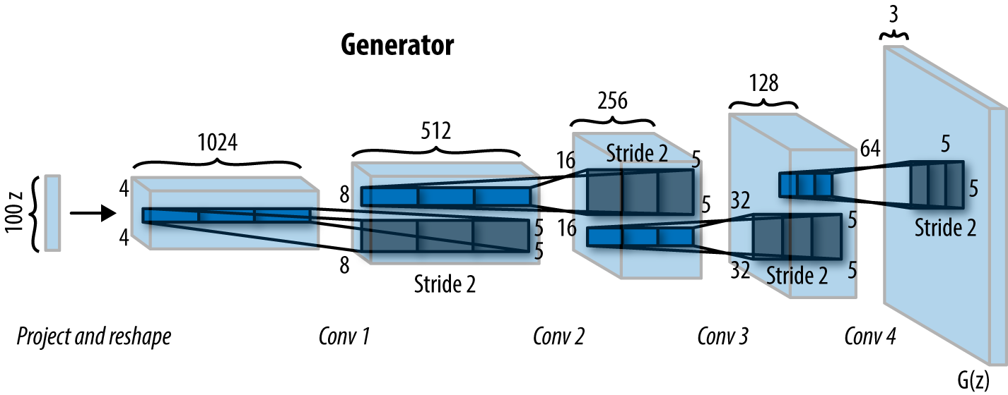
Here, we are doing the same thing as the discriminator, just in the other direction. First, we take our input, called Z, and feed it into our first deconvolutional layer. Each deconvolutional layer performs a deconvolution and then performs batch normalization and a leaky ReLu as well. Then, we return the tanh activation function.

Off to training!

Before we can actually kick off the training process, we need to do some other things. First, we need to define all variables that help us calculate the losses. Then, we need to define our optimization function. Finally, we are going to build a little function to output the generated images and then train the network.

Loss Functions

Rather than just having a single loss function, we need to define three: The loss of the generator, the loss of the discriminator when using real images, and the loss of the discriminator when using fake images. The sum of the fake image and real image loss is the overall discriminator loss.

First, we define our loss for the real images. For that, we pass the output of the discriminator when dealing with real images and compare it with the labels, which are all 1, which means true. We use a technique called label smoothing here to help our network getting more accurate by multiplying the 1s with 0.9.

Then, we define the loss for our fake images. This time we pass in the output of the discriminator when dealing with fake images and compare it to our labels, which are all 0, which means they are fake.

Finally, for the generator loss, we do the same like in the last step, but instead of comparing the output with all 0s, we compare it with 1s, since we want to fool the discriminator.

Optimization and Visualization

In the optimization step, we are looking for all variables that can be trained by using the tf.trainable_variables function. Since we used variable scopes before, we can very comfortably retrieve these variables. We then use the Adam optimizer to minimize the loss for us.

def model_opt(d_loss, g_loss, learning_rate, beta1):
    """
    Get optimization operations
    """
    t_vars = tf.trainable_variables()
    d_vars = [var for var in t_vars if var.name.startswith('discriminator')]
    g_vars = [var for var in t_vars if var.name.startswith('generator')]

In the last step of our preparation, we are writing a small helper function to display the generated images in the notebook for us, using the matplotlib library.

Training

We are at the last step! Now, we just get our inputs, losses, and optimizers which we defined before, call a TensorFlow session and run it batch per batch. Every 400 batches, we are printing out the current progress by showing the generated image and the generator and discriminator loss. Now lean back and see the faces show up slowly but steady. This progress can take up to an hour or more, based on your setup.

Conclusion

Congratulations! You know now what GANs do and even know how to generate images of human faces using them. You might ask: “What do I need this for? I will never have to generate images of random faces.” While that might be true, GANs have many other applications.

Researchers at the University of Michigan and the Max Planck Institute in Germany used GANs to generate images from text. They were able to generate extremely real looking flowers and birds based on written descriptions. This could be extended to something very useful, like police sketches or graphic design.

Researchers at Berkeley also managed to create a GAN that enhances blurry images and even reconstructs corrupted image data.

GANs are extremely powerful and who knows—maybe you will invent their next groundbreaking application.

This post is a collaboration between O’Reilly and TensorFlow. See our statement of editorial independence.