Contouring learning rate to optimize neural nets
Tips and tricks for treating learning rate as a hyperparameter, and using visualizations to see what’s really going on.
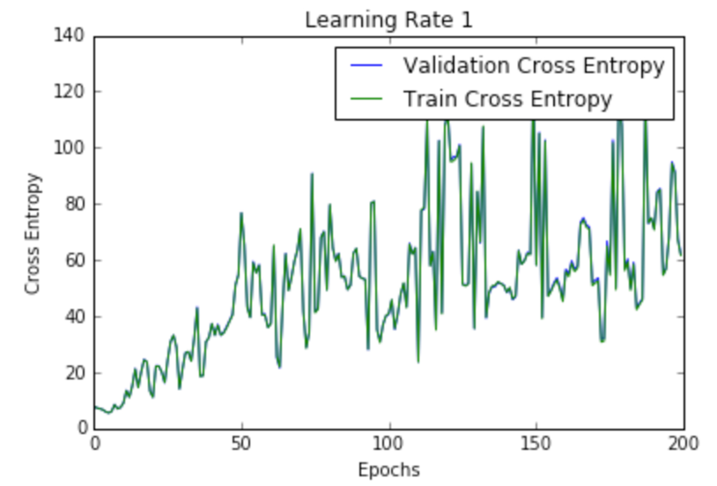 Cross entropy loss per epoch curve at Learning Rate 1 (source: Siddha Ganju, used with permission)
Learning rate is the rate at which the accumulation of information in a neural network progresses over time. The learning rate determines how quickly (and whether at all) the network reaches the optimum, most conducive location in the network for the specific output desired. In plain Stochastic Gradient Descent (SGD), the learning rate is not related to the shape of the error gradient because a global learning rate is used, which is independent of the error gradient.
However, there are many modifications that can be made to the original SGD update rule that relates the learning rate to the magnitude and orientation of the error gradient.
Why contour the learning rate?
Contouring the learning rate over time is similar to contouring the speed of a car according to road conditions. On smooth, broad roads such as a highway, we can increase our speed (learning rate), but on narrow, hilly, or valley roads, we must slow down. Additionally, we don’t want to drive too slowly on highways, or we’ll take too long to reach the destination (longer training time because of improper parameters). Similarly, we don’t want to drive too fast on hilly and narrow roads (like ravines in the optimization loss surface), because we could easily lose control of the car (be caught in jitter, or create too much bounce with little improvement) or skip the destination (the optima).
Keep in mind that “…a high learning rate… [indicates] the system contains too much kinetic energy and the parameter vector bounces around chaotically, unable to settle down into the deeper, but narrower parts of the loss function” (see Karpathy’s Notes for cs231n).
From the same source, a good guesstimate for an initial learning rate can be obtained by training the network on a subset of the data. The ideal strategy is to start with a large learning rate and divide by half until the loss does not diverge further. When approaching the end of training, the decay of the learning rate should be approximately 100 or more. Such decay makes the learned network resistant to random fluctuations that could possibly reverse the learning. We’ll start with a small LR, test out on a small set of data, and choose the appropriate value.
Learning rate decay
Non-adaptive learning rates can be suboptimal. Learning rate decay can be brought about through reducing decay by some constant factor every few epochs, or by exponential decay, in which the decay takes a mathematical form of the exponential every few epochs. “Decay” is often considered a negative concept, and in the current case of learning rate decay it’s a negative, too: it refers to how much the learning rate is decreasing. However, the result of this kind of decay is actually something we very much want. In a car, for instance, we decrease the speed to suit the road and traffic conditions; this deacceleration can be understood as a “decay” in the velocity of the car. Similarly, we gain benefits from decaying the learning rate to suit the gradient.
Decreasing the learning rate is necessary because a high learning rate while proceeding into the training iterations has a high probability to fall into a local minima. Think of a local minima as a speeding ticket, a toll or traffic light, or traffic congestion—something that basically increases the time taken to reach the destination. It’s not possible to completely avoid all traffic lights and tolls, but there is an optimal route that we prefer while driving. Similarly, in training we want to avoid the zig-zag bouncing of the gradient while looking for the optimal route and prefer training on that path. Ideally, we don’t want to speed up too much because we’ll get a speeding ticket (jump into a local minima and get stuck). The same analogy applies to learning rates.
Momentum is an adaptive learning-rate method parameter that allows higher velocity to collect along shallow directions, and lower velocity along steep directions. This definition of momentum is considered “classical momentum,” in which a correction is applied to the velocity and then a big jump is taken in the direction of the velocity. Momentum helps to accelerate or decelerate the base learning rate with respect to the changing gradient, causing a change in the net speed of the learning rather than its location on the loss surface. Momentum makes the learned network more resistant to noise and randomness in the inputs.
Other update rules that treat learning rate as a hyperparameter include:
- The AdaGrad update by Duchi et al., 2011, adds an element-wise scaling of the gradient based on the historical sum of squares in each dimension.
- The RMSProp adaptive learning rate by Tieleman and Hinton, 2012, keeps a moving average of the squared gradient for each weight to normalize the current gradient. RMSProp adds more resistance to fluctuations and random noise.
- The Adam update by Kingma and Ba, 2014, introduces a bias correction compensating for the zero initialization.
- And rprop, which uses only use the sign of the gradient to adapt the step size separately for each weight. This should not be used on mini-batches.
Apart from these rules, there are the very computation-heavy second order methods that follow Newton’s update rule. The second order methods do not treat learning rate as a hyperparameter, however; due to their high computational demands, they are rarely used in large-scale deep learning systems.
Figure 1 shows the comparison of different optimization techniques under similar hyperparameter settings:
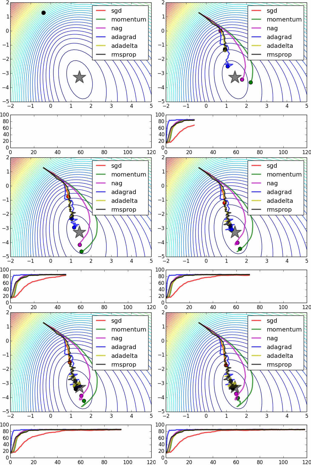
In this image, the momentum update overshoots the target, but reaches the overall minimum faster. “NAG” is the Nesterov Accelerated Gradient, in which the first step is taken in the direction of the velocity and then a correction is made to the velocity vector based on the new location.
Essentially, we aim not to fall into decay, but to use the decay to fall into the right place. It is imperative to selectively increase or decrease learning rate as training progresses in order to reach the global optimum or the desired destination. Don’t be afraid of this because we often have to do it again and again.
Visualizations
Visualizations are necessary to know how the learning is progressing. A loss versus epochs plot, for instance, is very useful to understand how the loss is changing with the epochs. An epoch is completed when all data points have been seen at least once in the current run. It’s preferable to track epochs in comparison to iterations, because the number of iterations depends on the arbitrary setting of batch size.
A good way to generate this plot is by overlaying the loss per epoch curve for different sets of parameters. This process helps us to recognize the set of parameters that works best for the training at hand. These plots have loss along the y axis and number of epochs along the x axis. Overall, the loss curves shown in Figure 2 look similar, but there are slight differences in their optimization patterns, represented in the number of epochs necessary for convergence and the resultant error.
There are many kinds of loss functions, and selecting which one to use is an important step. For some classification tasks, the cross entropy error tends to be more suitable than other metrics, such as the mean squared error, because of the mathematical assumptions behind the cross entropy error. If we view neural networks as probabilistic models, then, cross entropy becomes an intuitive cost function with its sigmoid or softmax nonlinearity which maximizes the likelihood of classifying the input data correctly. The mean square error, on the other hand, focuses more on the incorrectly labeled data. The mean classification error thus becomes a crude yardstick.
Cross entropy’s niceties include a log term, making it more granular, while taking into account the closeness of the predicted value with the target. Cross entropy also has nicer partial derivatives producing larger errors, which lead to larger gradients that ensure quicker learning. Generally, the cost function should be picked based on the assumptions that match the output units and the probabilistic modelling assumptions. For instance, a softmax and cross entropy serve best for multiclass classification. Plotting the cross entropy function might be more interpretable due to the log term simply because the learning process is mostly an exponential process taking the form of an exponential shape.
Experimenting with different learning rates
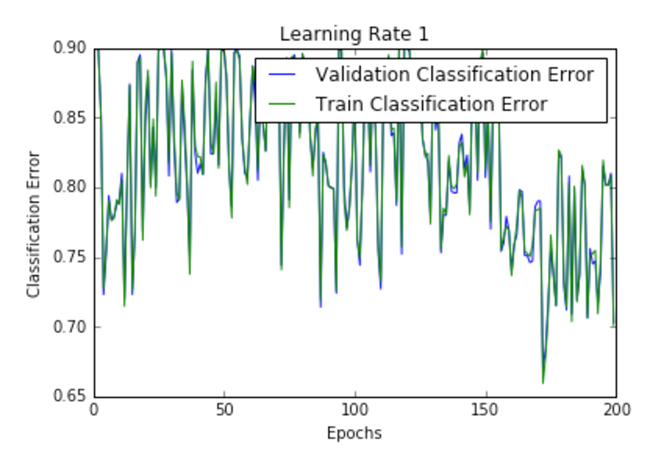
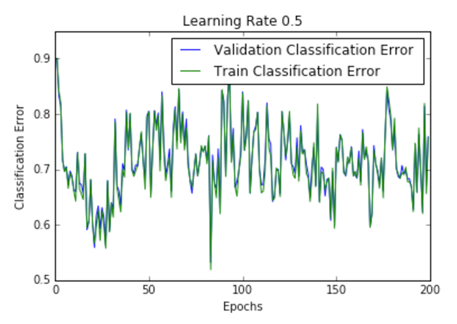
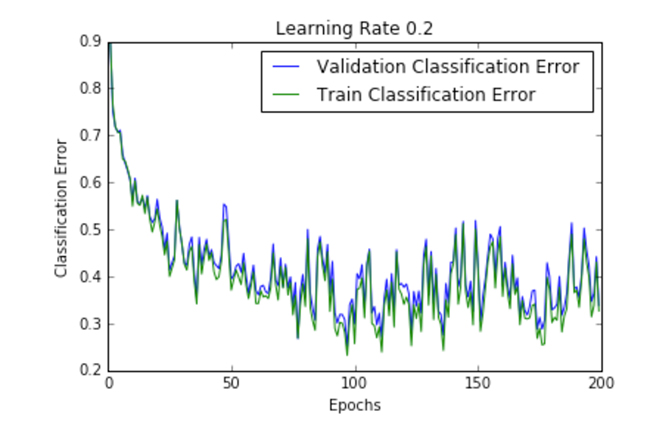
Learning rate is a hyperparameter that controls the size of update steps. As the learning rate increases, the number of oscillations increase. As seen in the plots of Figure 2, there is a lot of confusion or random noise with an increase in the learning rate. All the plots in Figure 2 are for a one-layer neural network trained on the MNIST data set.
We can infer from the plots that a high learning rate is more likely to blow up the whole model, resulting in numerical instability such as overflows or underflows, which was also empirically noted while running these experiments. In fact, NAN’s started appearing just after the first training epoch.
| Learning Rate | Cross Entropy | Classification Error |
|---|---|---|
| 1 |  |
 |
| .5 | 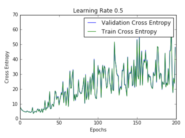 |
 |
| .2 | 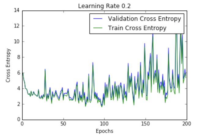 |
 |
| .1 |  |
 |
| .01 | 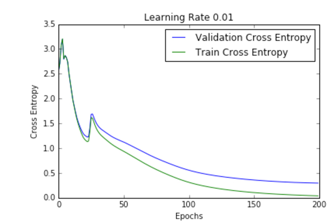 |
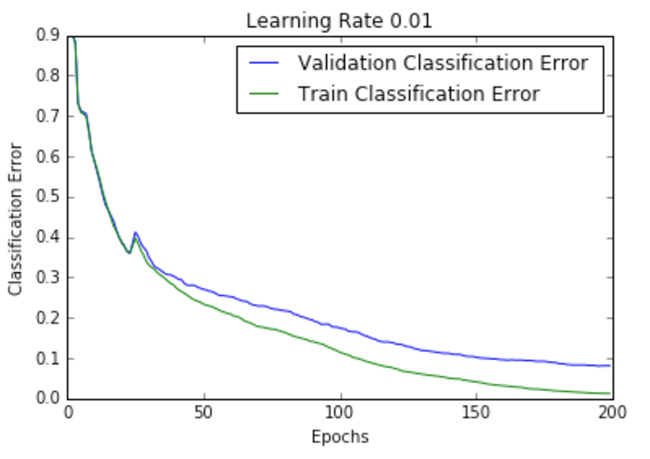 |
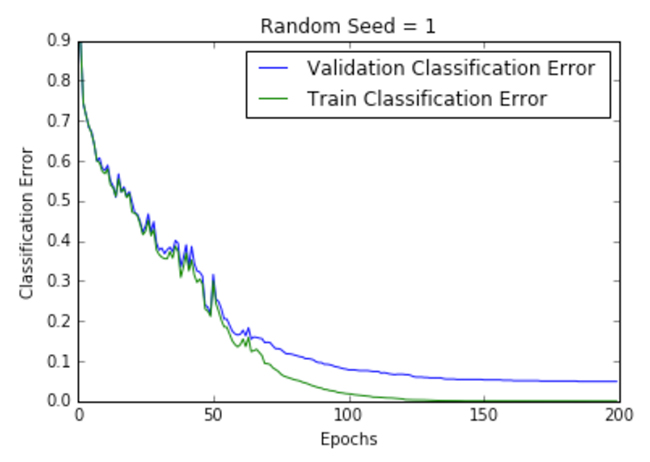
Figure 2 shows the loss per epoch curve for different learning rates. Two different loss functions, the cross entropy and the classification error, are compared. The plots show that at lower learning rates, the improvements are linear (Learning rate .01). When the learning rates are high, almost exponential jumps are seen (Learning rate 1 and .5). The higher learning rates are capable of decaying the loss much faster, but the disadvantage is that a big jump might land them in a local minima, and then get stuck at worse values of loss.
This phenomenon is often seen as oscillations in the plots, indicating that the parameters that were learned are mostly bouncing around, and not able to settle and make the gradient move towards the global min. If the validation curve closely follows the training curve, the network has trained correctly. However, large gaps between the validation and training curves indicate that the network is overfitting on the training set (Learning rate .01). Chances of overfitting can be reduced by using dropout or other regularization techniques.
Use a separate, adaptive learning rate for each connection
It is common to have networks with more than one layer. Each layer has a different fan-in or the number of inputs, that determines the overshoot effect caused by simultaneously updating the incoming weights of a unit aimed at correcting the same error (as is the case in the global learning rate). Additionally, the magnitudes of the gradients vary for different layers, especially if the initial weights are small (always the case for initialization). Hence, the appropriate learning rates can vary widely between weights.
A fix for this issue involves setting a global learning rate and multiplying it by an appropriate local gain that is determined empirically for each weight. In order to enhance performance of the network, the gains should lie in a reasonable predefined range. While using separate adaptive learning rates, either the entire batch should be used for learning, or larger mini-batches should be used in order to ensure the changes in the signs of the gradients are not mainly due to the sampling error of a mini-batch or random fluctuations. These per-weight adaptive learning rates can also be combined with momentum. (For more information, see Lecture 6b, Neural Networks, Coursera.)
Learning rate for transfer learning
Transfer learning is modifying an existing pretrained model for use in another application. This reuse of models is necessary because it is relatively rare for a sizable data set for training purposes to exist in the application domain. Fine-tuning is a type of transfer learning in which a slice of the network, like the last layers of a network are modified to give the application-specific number of outputs. There are other types of transfer learning methods which we do not discuss here. As Figure 3 demonstrates, fine-tuning modifies a network to learn a slightly different kind of data (such as the accordion) when the network has already been trained on a similar kind of data (the piano).

As the network is pretrained, fine-tuning takes considerably less time to train, because the network has already acquired most of the information it needs and must only refine that knowledge during the fine-tuning phase.
While fine-tuning, we decrease the overall learning rate while boosting the learning rate for the slice (last layer or the new layer). For example, in the open source Caffe framework, the base_lr should be decreased in the solver prototxt, while the lr_mult for the newly introduced layer should be increased. This helps to bring about a slow change in the overall model but an expeditious change in the new layer utilizing the new data. The rule of thumb is to keep the learning rate for the layer being learned at least 10 times more than the other static layers (the global learning rate).
Conclusion
In this article, we only briefly touched on a few things out of all the parameters in the parametric-multiverse of deep learning algorithms. The decay of learning rate is one such parameter, and is essential to avoid taxing local minimas. While performing your deep learning experiments, remember to make exhaustive use of visualizations. They are one of the most important ways to understand what’s really happening inside a deep learning black box.
Imagine deep learning as full of little knobs and switches, like a pilot’s dashboard. We need to learn how to tweak these to get the best outputs for the work at hand. We can always find a pre-trained model for the application we are developing, selectively add or delete parts of it, and ultimately fine-tune it for the application we need. And, if we contour our learning rate accurately, we reach our destination in good time.
