A look at deep learning for science
Scientific use cases show promise, but challenges remain for complex data analytics.
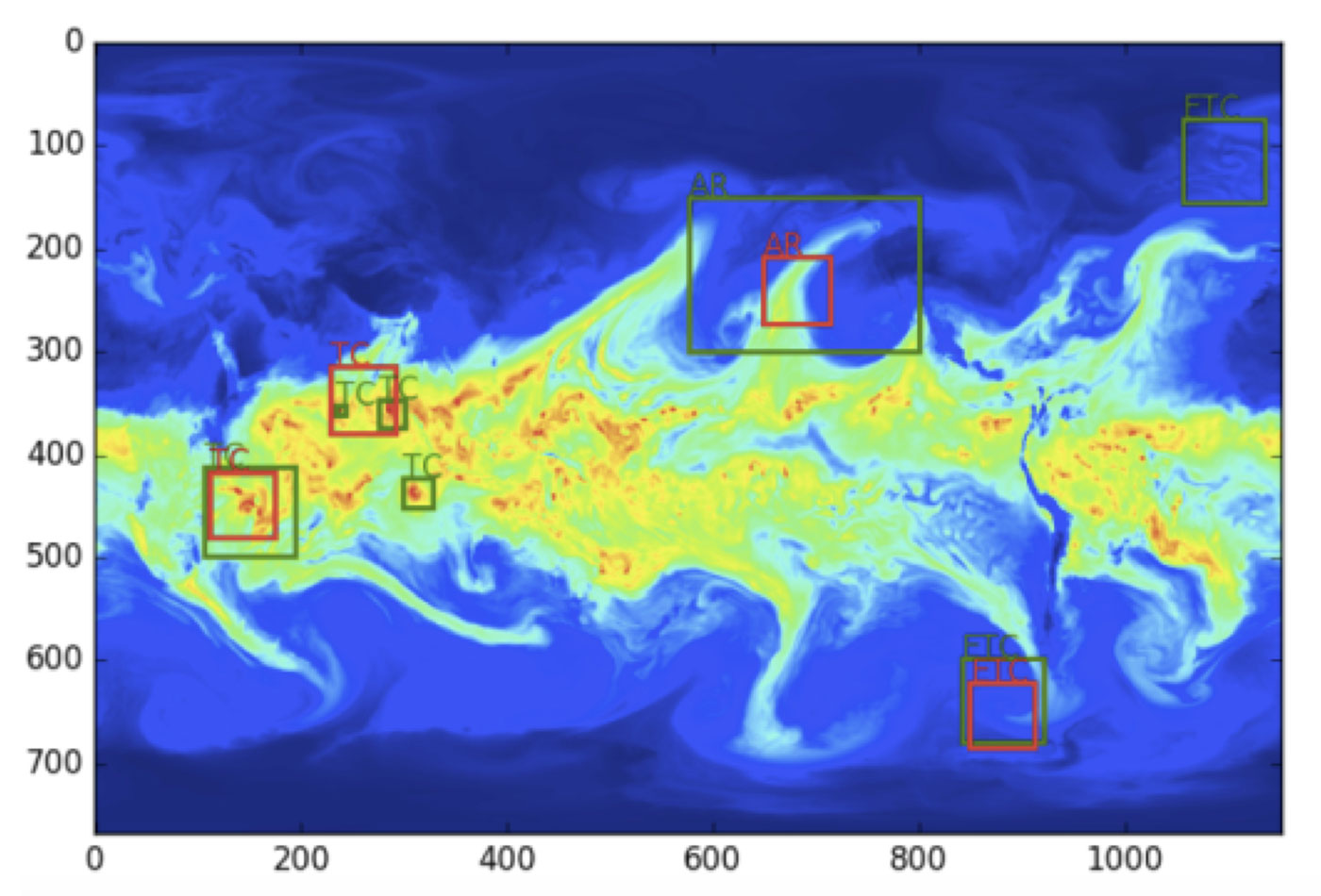 Sample results (ground truth: Green, DL prediction: red) for weather patterns and their location. (source: Courtesy of Evan Racah, LBNL, used with permission.)
Deep learning is enjoying unprecedented success in a wide variety of commercial applications. Around 10 years ago, very few practitioners could have predicted that deep learning-powered systems would surpass human-level performance in computer vision and speech recognition tasks. At Lawrence Berkeley National Laboratory, we are confronted with some of the most challenging data analytics problems in science. While there are similarities between commercial and scientific applications in terms of the overall analytics tasks (classification, clustering, anomaly detection, etc.), a priori, there is no reason to believe that the underlying complexity of scientific data sets would be comparable to ImageNet. Are deep learning methods powerful enough to produce state-of-the-art performance for scientific analytics tasks? In this article, we present a number of case studies, chosen from diverse scientific disciplines, that illustrate the power of deep learning methods for enabling scientific discovery.
Related to these topics, I recently chatted with O’Reilly’s Jon Bruner on the Bots Podcast. We discussed the architecture of the LBNL supercomputing center, the push to integrate deep learning libraries within this architecture, and some compelling use cases for deep learning methods (such as object or pattern detection) that must scale for extremely large data sets. You can listen to the audio of our interview below (or download from iTunes here):
Galaxy shape modeling with probabilistic auto-encoders
Contributors: Jeffrey Regier, Jon McAullife
Galaxy models have numerous applications in astronomy. For example, a slight distortion in a galaxy’s appearance may indicate the gravitational pull of nearby dark matter. Dark matter is hypothesized to be five times as common as ordinary matter, but there is no consensus on whether it exists. Without a model of what a galaxy looks like unaltered, there is no basis for concluding that a distortion is present.
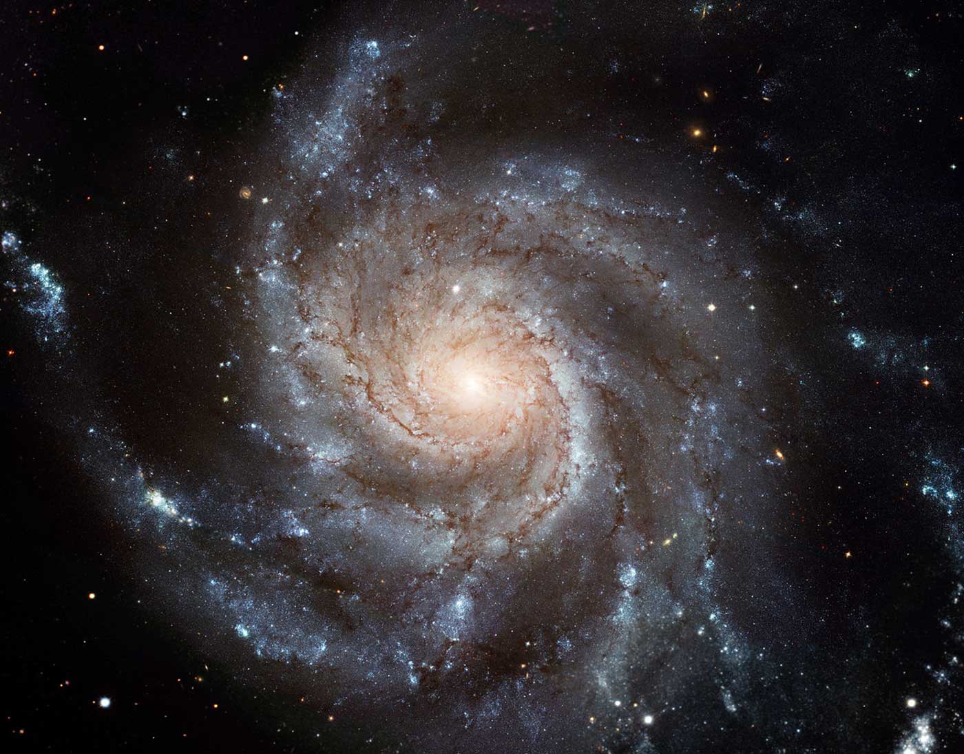
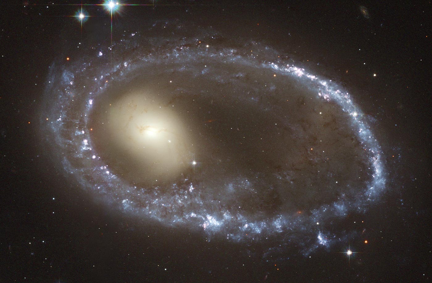
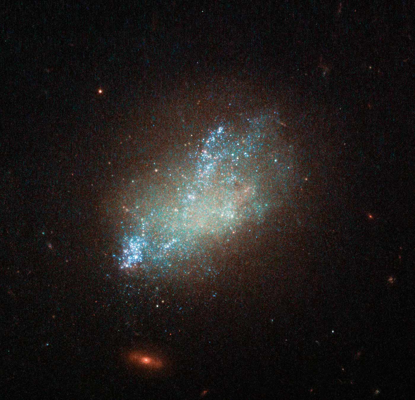
Because galaxies have much in common, a model fit to a sample of galaxies can accurately represent the whole population of galaxies. Shared characteristics include spiral “arms” (see Figure 1 below), rings (Figure 2), and brightness that decreases with distance from the center—even among irregular galaxies (Figure 3). These commonalities are high-level features, not easily described at the level of individual pixels.
To date, most neural-network successes have been on supervised learning problems: given an input, predict an output. If the predicted output does not match the correct answer, adjust the network’s weights. For galaxy models, there is no correct output. Rather, we seek a probabilistic model of images that assigns high probability to images of galaxies, while assigning a total probability of one to all possible images. A neural network specifies a conditional probability within this model.
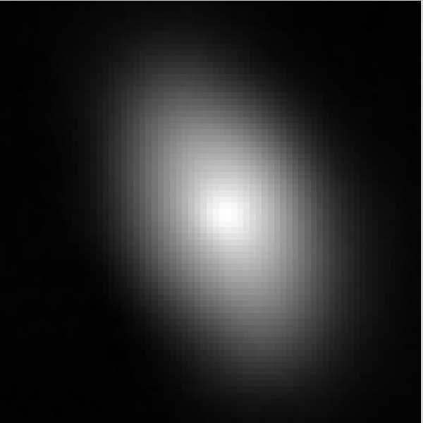
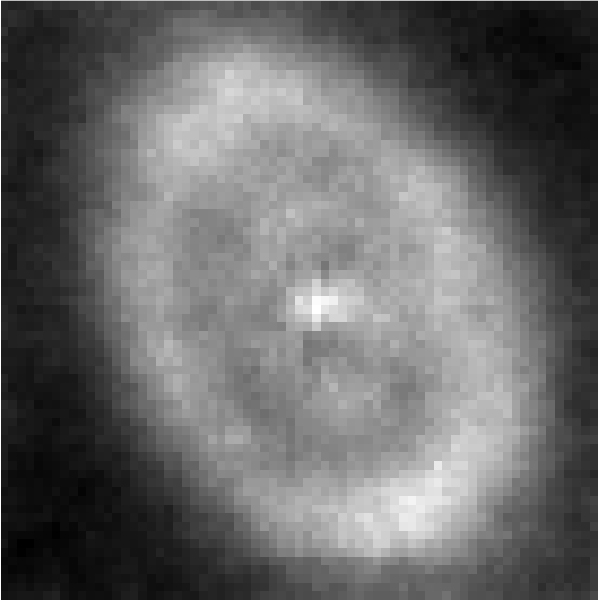
In the probabilistic model, an unobserved random vector $z$ is drawn from a multivariate standard normal distribution. A neural network maps $z$ to a mean and a covariance matrix that parameterize a high-dimensional multivariate normal distribution, with one dimension per pixel of a galaxy image. The neural network may have as many layers and nodes as are helpful for representing the map. Figure 4 shows the mean of a multivariate normal distribution for a particular galaxy image, and Figure 5 shows the diagonal of the covariance matrix. Finally, a galaxy image is sampled from this multivariate normal distribution.
One may take either of two perspectives on our procedure for learning the weights of the neural network from galaxy images: algorithmic and statistical. Algorithmically, our procedure trains an autoencoder. The input is an image, the low-dimensional $z$ vector is a narrow layer in the middle of the network, noise is added, and the output is a reconstruction of the input. The loss measures the difference between the input and the output. Our choice of loss function and the type of noise we add to the autoencoder, however, follow from the statistical model. With these choices, training the autoencoder is equivalent to learning an approximate posterior distribution on the unobserved vector $z$, through a technique called ”variational inference.” The posterior distribution for a galaxy tells us what we want to know: how the galaxy most likely appears (i.e., the posterior’s mode) and the amount of uncertainty about its appearance. It combines our prior knowledge of what galaxies generally look like with what we learn about a particular galaxy from its image.
We implemented the proposed variational autoencoder (VAE) using Mocha.jl, a neural network framework in Julia based on Caffe. We trained our model with 43,444 galaxy images, each cropped around one prominent galaxy and downscaled to 69 x 69 pixels. On 97.2% of galaxy images in a hold-out set, the proposed VAE assigns higher probability to the image than the current common practice of modeling galaxies with bivariate Gaussian densities.
Finding extreme weather events in climate simulations
Contributors: Evan Racah, Christopher Beckham, Tegan Maharaj, Yunjie Liu, Chris Pal
Extreme weather events pose great potential risk on ecosystem, infrastructure, and human health. Analyzing extreme weather in the observed record (satellite and weather station products) and characterizing changes in extremes in simulations of future climate regimes is an important task. Typically, the climate community specifies patterns through hand-coded, multivariate threshold conditions. Such criteria are usually subjective, and there is often little agreement in the community on the specific algorithm that should be used. We have explored a completely different paradigm, namely that of training a deep learning-based system on human ground-truth labeled data, to learn pattern classifiers.
Our first step was to consider the problem of supervised classification for centered, cropped patches of tropical cyclones and atmospheric rivers. We identified 5,000-10,000 patches and trained a vanilla convolutional network (in Caffe) with hyperparameter tuning (in Spearmint). We observed 90-99% classification accuracy for the supervised classification task. The next step was to consider a unified network that could simultaneously perform pattern classification for multiple types of patterns (tropical cyclones, atmospheric rivers, extra-tropical cyclones, etc.) and localize these patterns with a bounding box. This is the more advanced, semi-supervised formulation of the problem. Our current network is depicted in Figure 6.

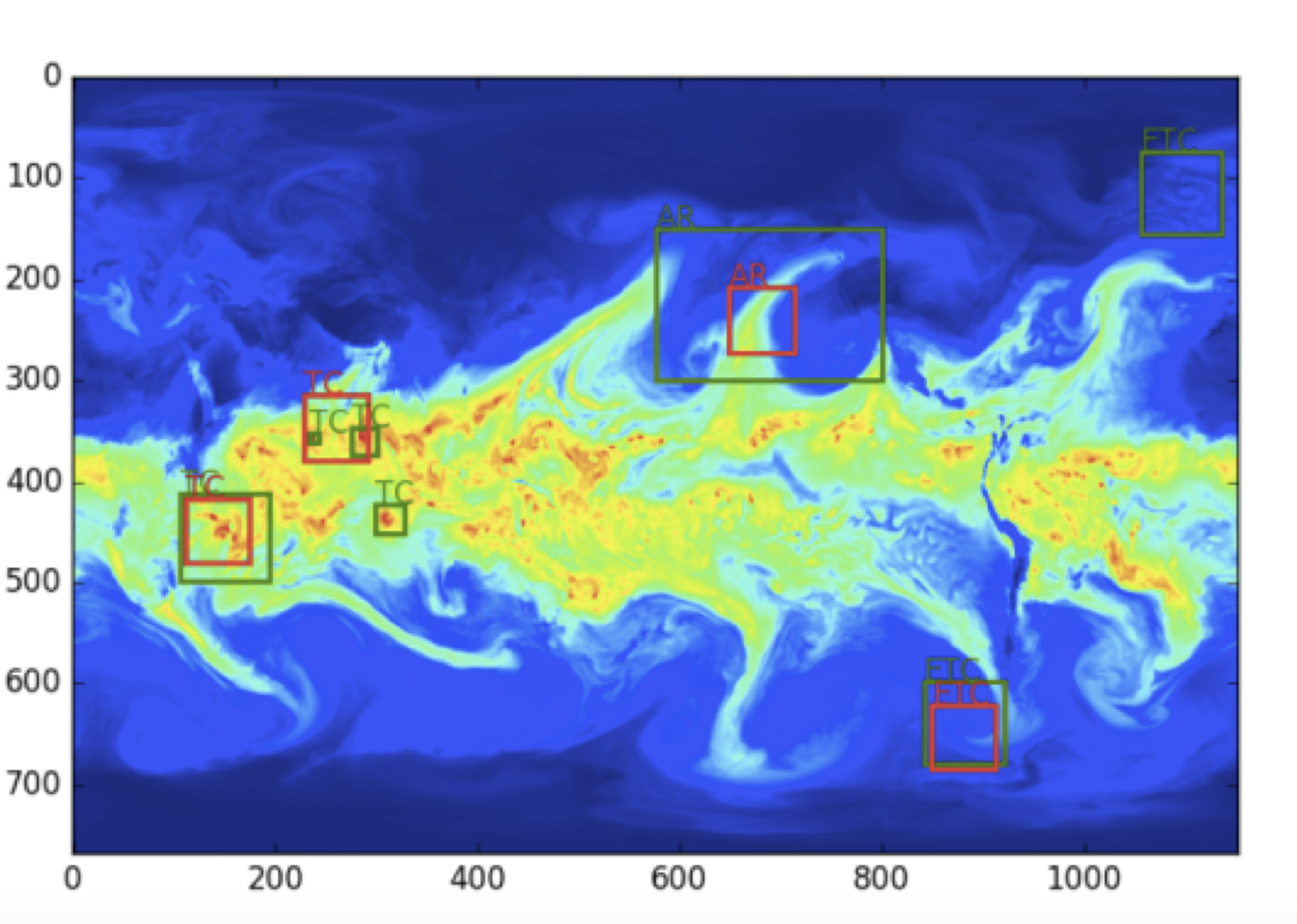
Figure 7 highlights some of the sample results obtained by the semi-supervised architecture. While further tweaks on the architecture are ongoing, t-SNE plots of the underlying clusters reveal that the method has the capability to discover new coherent fluid flow structures in the data set. The current architecture operates on instantaneous snapshots; we are extending the model to incorporate time explicitly to make more accurate predictions.
Learning patterns in cosmology mass maps
Contributors: Debbie Bard, Shiwangi Singh, Mayur Mudigonda
Upcoming astronomical sky surveys will obtain measurements of tens of billions of galaxies, enabling precision measurements of the parameters that describe the nature of dark energy, the force that is accelerating the expansion of the universe. For example, maps can be constructed of the matter in the universe—regular matter and dark matter—using the technique of gravitational lensing. Characterizing these mass maps allows us to distinguish between different theoretical models of dark energy.
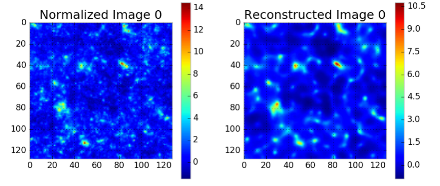
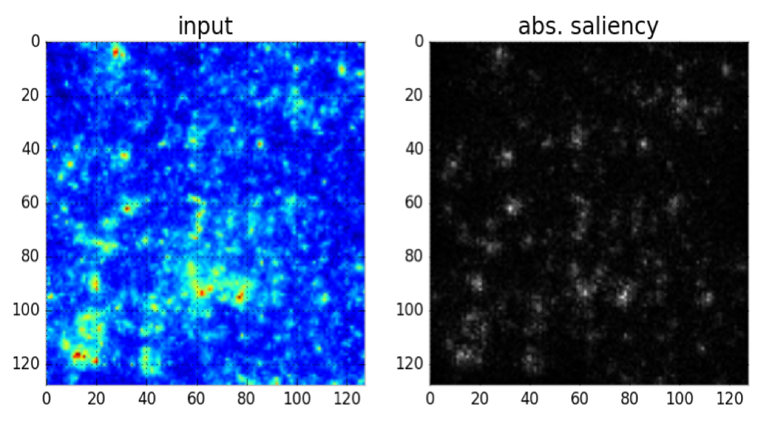
We explore emerging deep learning techniques to identify new ways of rapidly analyzing cosmological map data. These models offer the potential to identify unexpected features in mass maps that give new insight into the structure of the universe. We developed an unsupervised Denoising Convolutional Autoencoder model in order to learn an abstract representation directly from our data. This model uses a convolution-deconvolution architecture, which is fed with input data from simulations of a theoretical universe (corrupted with binomial noise to prevent over-fitting). We use four convolutional layers, two bottleneck layers, and four deconvolution layers, implemented using the Lasagne package. It is trained using 10,000 images of mass maps, each 128×128 pixels. Our model effectively trains itself to minimize the mean-squared error between the input and the output using gradient descent, resulting in a model that, theoretically, is broad enough to tackle other similarly structured problems. Using this model, we were able to successfully reconstruct simulated mass maps and identify the structures in them (see Figure 8). We also determined which structures had the highest “importance” (i.e., which structures were most typical of the data, see Figure 9). We note that the structures of highest importance in our reconstruction were around high mass concentrations, which correspond to massive clusters of galaxies.
We also developed a supervised Convolutional Neural Network (CNN) with four hidden layers for classification of cosmological mass maps from two different simulated theoretical models. The CNN uses a softmax classifier, which minimizes a binary cross-entropy loss between the estimated distribution and true distribution. In other words, given an unseen convergence map, the trained CNN determines probabilistically which theoretical model fits the data best. Trained using 5,000 maps (128×128 pixels) from two theoretical models, this preliminary work demonstrates that we can classify the cosmological model that produced the convergence maps with 80% accuracy (see Figure 10).
Decoding speech from human neural recordings
Contributors: Jesse Livezey, Edward Chang, Kristofer Bouchard
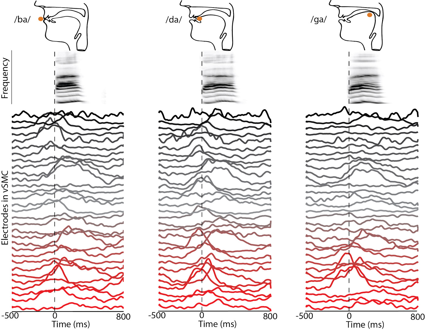
The seemingly effortless ability to produce the complex grammatical structures and acoustic patterns that comprise speech is unique to the human species. The seminal work of Penfield and Boldrey in the 1930s showed that different parts of the body (including the vocal tract) are represented in spatially localized areas in the brain. How the brain generates temporal patterns of neural activity, like those seen in Figure 11, across a set of interconnected brain areas to orchestrate the articulators of the vocal tract remains an open question.
Brains are composed of nonlinear processing elements (neurons), which exhibit a general hierarchical organization as signals are successively processed. Therefore, we posited that the hierarchical and nonlinear processing of deep neural networks (DNNs) would be well matched to the complex neural dynamics of speech production. On large (millions of examples), complex data sets, DNNs have demonstrated their ability to outperform traditional methods across many tasks. However, this improvement has not been demonstrated on neuroscience analytics tasks, which typically have much smaller (thousands of examples) data sets.
In recent work, we found that, even on the relatively small data sets typically attained in neuroscience experiments, DNNs outperform traditional methods for decoding (i.e., translating) brain signals into produced speech, attaining state-of-the-art speech classification performance (up to 39% accuracy, 25x over chance). Additionally, the performance of DNNs scales better than traditional classifiers as the training data set size grows, maximizing the return on relatively limited, but highly valuable data. The input data set comprised of 85 channels and 250 time-sample signals, which is classified into 1-of-57 categories. Data sets for an individual subject typically only have about 2,000 training examples, necessitating extensive hyperparameter search for best performance. The best networks had one or two hidden layers with hyperbolic-tangent nonlinearities, and were trained on GPUs and CPUs using the Theano library. Each model trained relatively quickly (30 minutes), but hundreds of models were trained during hyperparameter search. These results suggest that DNNs could become the state-of-the-art for brain-machine interfaces in the future, and that more work is needed to develop best practices for training deep networks on small data sets.
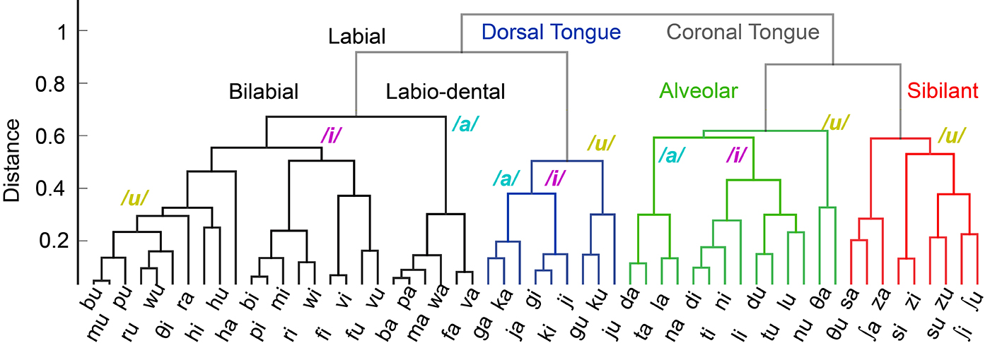
Beyond their capabilities to decode brain signals, which is critical for prosthetic purposes, we also investigated the utility of DNNs as an analytical tool to reveal structure in neuroscience data. We found that DNNs were able to extract a rich hierarchy of cortical organization during speech from noisy single-trial recordings. The extracted hierarchy (see Figure 12) provides insight into the cortical basis of speech control. We expect deep learning’s application to data analysis problems in neuroscience to grow as larger and more complex neural data sets are collected.
Clustering Daya Bay data with denoising autoencoders
Contributors: Samuel Kohn, Evan Racah, Craig Tull, Wahid Bhimji
The Daya Bay Reactor Neutrino Experiment searches for physics beyond the Standard Model of Particle Physics by measuring properties of antineutrinos, elementary subatomic particles produced by beta-decay in a nuclear reactor. Physicists monitor the light produced in large tanks of a detector medium, called liquid scintillator, looking for the characteristic double flash of light coming from an antineutrino interaction. Other background processes also produce flashes of light. Some backgrounds, such as cosmic-ray muons, are easy to identify, but others (like decays of Lithium-9 isotopes produced by the muons) closely mimic the neutrino signal. Separating the antineutrino signal from backgrounds is a difficult task; it can lead to systematic uncertainty and a reduction in signal efficiency as real antineutrino events are inadvertently rejected.
Currently, the Daya Bay analysis uses the time and total energy to discriminate signal from background. But there is information in the spatial distribution of light, which leaves open the possibility of better discrimination. By using unsupervised techniques from deep learning, we may learn the features that identify antineutrino events as distinct from Lithium-9 decays. With knowledge of the identifying features, we can update our current analysis cuts to enhance their discriminating power and improve the precision of our neutrino measurement.
The power of unsupervised deep learning is apparent in a case study performed to separate the antineutrino signal from a well-understood background caused by two uncorrelated flashes of light. In our case study, real data, rather than simulated data, was used to train the neural network. This is uncommon in supervised learning, but it works well in the unsupervised regime because it eliminates uncertainties and bias due to discrepancies between simulated and real data. A previous study used unsupervised learning to address a related signal-to-background problem at the Daya Bay experiment.
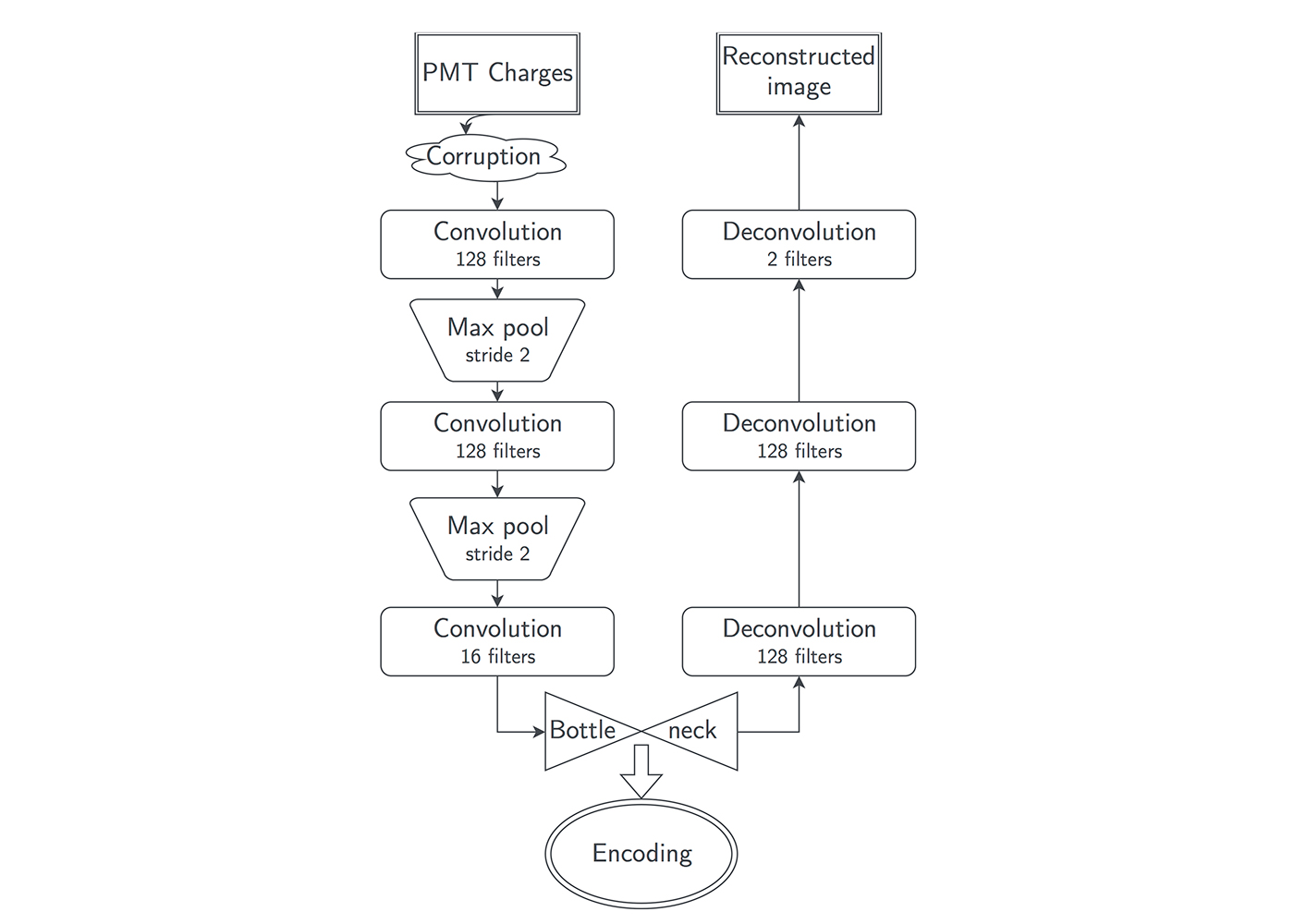
We used a denoising convolutional autoencoder neural network (Figure 13), which is characterized by three phases:
- the corruption phase, in which one-third of the image pixels are set to zero;
- the encoding phase, in which an image of the physics event is compressed into an encoding;
- and the decoding phase, in which an encoding is decompressed in an attempt to recover the original physics event image.
To successfully recover the original uncorrupted image, the autoencoder must learn how to infer missing information from the corrupted image it’s provided. When trained correctly, the autoencoder will create encodings that contain information on the important distinguishing features of the input images.
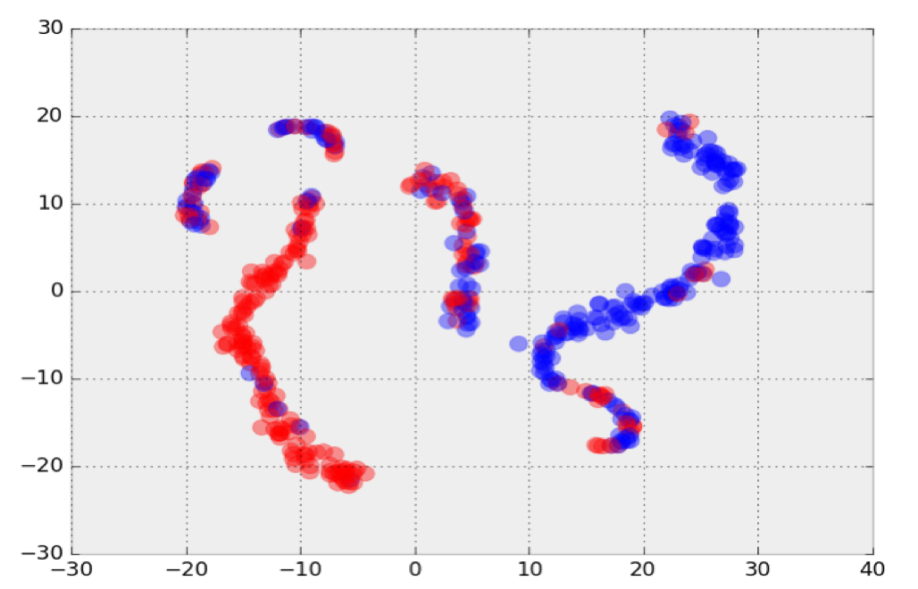
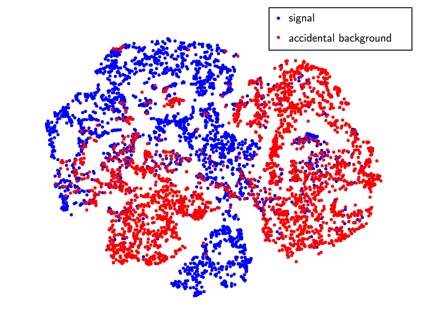
By using the t-SNE dimensional reduction algorithm, we can visualize the 16-dimensional encodings on the 2D cartesian plane. In Figure 14, it is clear that the neural network distinguishes our signal events from the accidental background—without being trained on individual event labels. This is a promising advance, which helps validate the use of an unsupervised neural network trained on real data. We will continue using our trial data set of accidental background events to improve the network architecture and determine which features are important to the neural network. After the technique is developed further, we will apply it to the physics problem of separating Lithium-9 background.
Classifying new physics events at the Large Hadron Collider
Contributors: Thorsten Kurth, Wahid Bhimji, Steve Farrell, Evan Racah
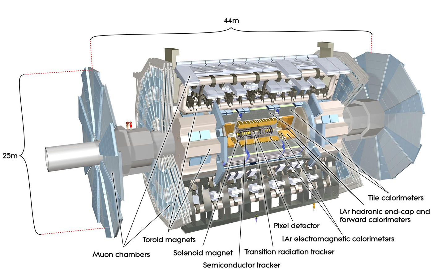
The Large Hadron Collider collides protons 40 million times per second at the highest energies ever achieved. Each collision produces sprays of resulting particles that are detected in instruments, such as the ATLAS detector (Figure 15), with hundreds of millions of channels of electronics attempting to discover new, previously unknown particles. The high luminosity upgrade of the LHC (HL-LHC) is expected to increase the rate of collisions by an order of magnitude. Data from the current detector already totals hundreds of petabytes. The only way to handle this volume and complexity of data is to rapidly filter away the bulk of it using both “triggers” on the detector and filters in offline data analysis. After triggers have down-sampled the data (to around 200 events per second), it is then reconstructed into objects such as particle tracks and energy deposits, reducing to hundreds of dimensions per event. This is then further down-sampled to analysis data, which has tens of dimensions depending on the particular physics of interest. Figure 16 shows a collision event illustrating some of these detector signals and the higher-level reconstructed objects.
The 2013 Nobel Prize in Physics for the theory of the Higgs Boson was a direct result of the detection of this particle at the LHC. The Higgs Boson completed the Standard Model of Particle Physics, and the exact nature of the new physics beyond the Standard Model is not well known. Therefore, the accuracy and speed of the triggering, reconstruction, and physics analysis algorithms directly impacts the ability of the experiment to discover new phenomena—more than ever before. It is already clear that the current approach and algorithms for filtering data will struggle to scale computationally to the next phase of the LHC, and they run the risk of overlooking more exotic new physics signals. It is therefore vital to explore innovative, efficient methods to tackle data filtering. Methods that apply machine learning to run a physics analysis at the scale and rates of the initial detector signals or raw data have the potential to make new discoveries that will change our understanding of fundamental physics.
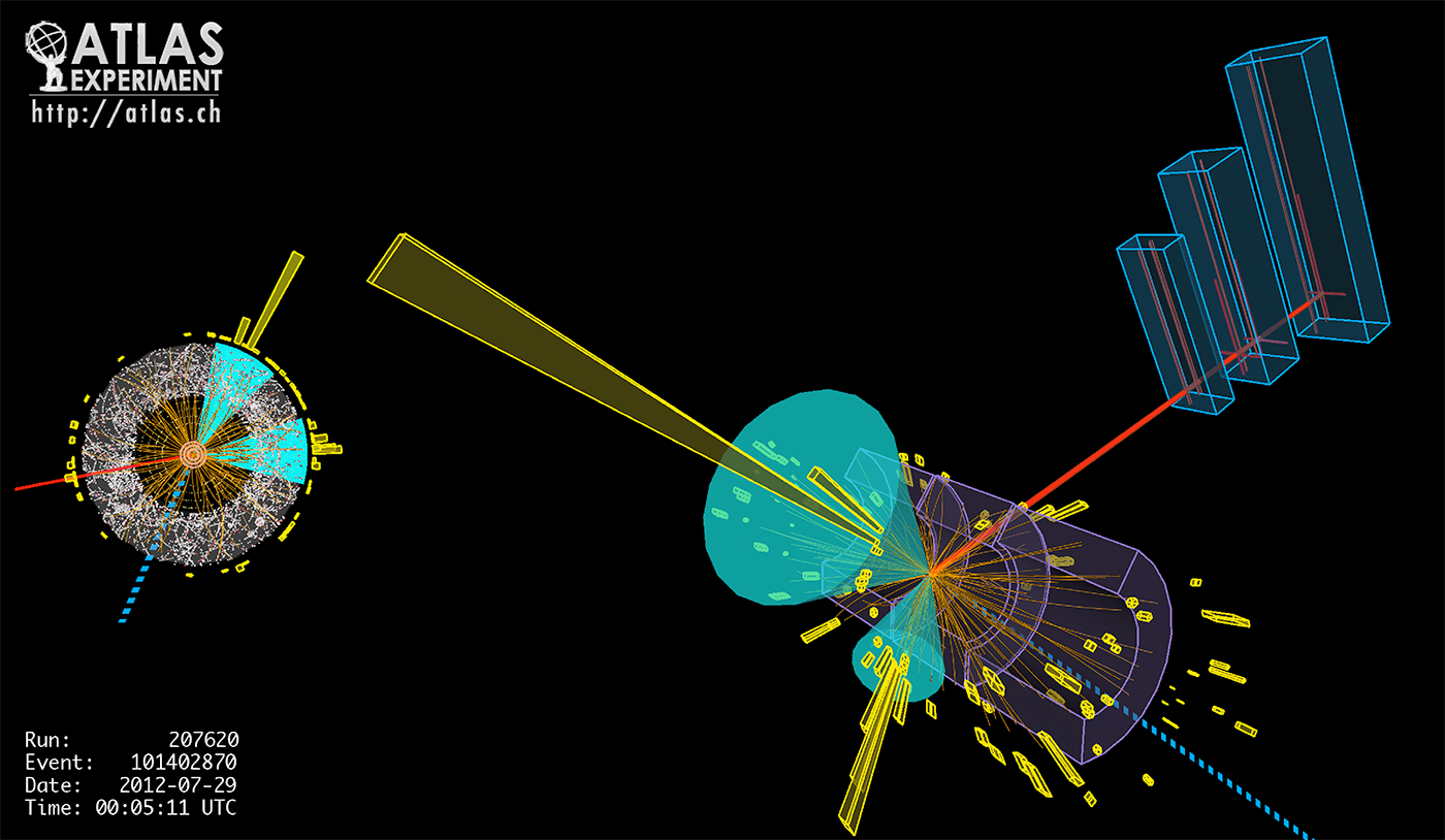
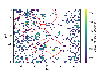
Deep learning offers the potential to learn novel selection filters to extract rare new physics signals that are more accurate than existing approaches, more flexible for alternative new physics signatures, and also computationally tractable to run on large dimensionality input data (corresponding to detector channels). We are exploring classifiers trained on simulations of new physics and well as anomaly detection algorithms that only use background (known Standard Model) samples for training. The signals that are output from particle physics detectors can be thought of as images (such as Figure 17), and therefore we exploit convolutional architectures. An example architecture, showing the layers of the neural network we use for classification is shown below.
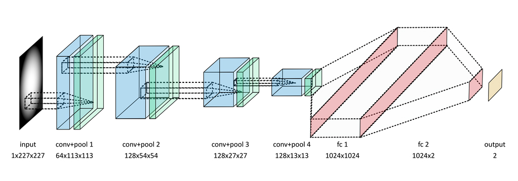
Our approach is novel in that it uses data from the detector before it has been reconstructed into high-level physics objects using high-resolution images (currently 227×227 pixels). This allows us to learn more sensitive patterns that may not be exploited by existing physics algorithms. Using large models and data sets requires scaling across multiple compute nodes, which is also novel for deep learning in this science domain.
We currently achieve classification performance in excess of the simple selections on high-level reconstructed features typically used for selecting this kind of physics, demonstrating the suitability of these kind of architectures. We are also scaling these architectures to large numbers of compute resources and beginning to explore anomaly detection that doesn’t require simulating the new physics of interest.
Open challenges
After having reviewed a number of practical applications of deep learning, we have converged on the following challenges (which are perhaps unique to the applied domain science context):
- Performance and scaling: Deep learning methods are computationally expensive. Our current experiments process 1-100GB-sized data sets, and take anywhere from one day to one week to converge on many-core architectures. This is prohibitive for hyperparameter tuning. There is a critical need to improve single-node performance for many-core architectures, and to scale networks using data and model parallelism on O(1000) nodes.
- Complex data: Scientific data comes in many shapes and sizes. 2D images can have anywhere from 3-1000 channels, 3D structured and unstructured grids are common, both sparse and dense data sets are prevalent in the field, and one can often find graph structures that encode key relationships. It is important that deep learning methods/software be able to operate on such data sets.
- Lack of labeled data: Scientists do not have ready access to vast amounts of high-quality, labeled images. Even if some communities were to self-organize and conduct labeling campaigns, it is unlikely we would have high-quality, ImageNet-style databases will millions of images. Much of domain science will always operate in the unsupervised (i.e., unlabeled data) or semi-supervised (i.e., limited labeled data for some classes) regimes. It is therefore very important that deep learning researchers continue to demonstrate compelling results in light of limited training data.
- Hyperparameter tuning: Domain science experts have limited intuition into the effect of tweaking network configurations (number and depth of convolutional layers); types of non-linear/pooling functions; learning rates; optimization schemes; training curricula, etc., for their specific problem. In order for deep learning to be broadly employed in science, it is important that we package capabilities for automatically tuning these hyperparameters.
- Interpretability: In contrast to commercial applications, where it is perhaps acceptable to have a black-box, near-perfect predictor, domain scientists need to understand and explain the function that the neural network is learning to the rest of their communities. They need to understand what features are being learned, whether the features are physically meaningful/insightful, and whether non-linear functions on the learned features are analogous to physical processes. In an ideal case, choices of functions and features would be constrained based on our understanding of domain sciences. Currently, this important link is missing, and we are hopeful that the next generation of deep learning researchers will try to bridge the interpretability gap.
Summary
We have presented a number of successful applications of deep learning from diverse scientific disciplines at Lawrence Berkeley National Laboratory as well as the open challenges. It would be fair to summarize our empirical experience with deep learning as being extremely encouraging. We believe it is simply a matter of time before deep learning will be explored (and adopted) by several domain science disciplines. We will caution that some domain sciences will make more rigorous demands on the theoretical foundations and properties of deep learning networks. We would like to encourage deep learning researchers to engage the domain science community as a rich source of interesting problems.
